Abstract
当前,针对基本搜索问题设计简洁数据结构的研究兴趣日益高涨(参见 [23] 及其参考文献)。其动机在于:当今可获取的电子数据呈指数增长,其增速甚至超过了当前计算机内存和磁盘存储容量的显著提升。空间压缩是一个具有吸引力的议题,因为正如多位学者所指出的(如 Knuth [15]、Bentley [5]),它与性能提升密切相关。在设计这些隐式数据结构时,目标是尽可能减少与输入数据一同保存的辅助信息,同时不显著降低最终的查询性能。然而,输入数据以其完整形式表示,因而未能利用其中可能存在的重复性。这些议题的重要性对程序员而言是众所周知的,他们通常运用各种技巧尽可能压缩数据,同时仍然获得良好的查询性能。不过,他们的方法本质上是一些启发式策略,其有效性仅由实验所验证。
📄 原文
There is an upsurging interest in designing succinct data structures for basic searching problems (see [23] and references therein). The motivation has to be found in the exponential increase of electronic data nowadays available which is even surpassing the significant increase in memory and disk storage capacities of current computers. Space reduction is an attractive issue because it is also intimately related to performance improvements as noted by several authors (e.g. Knuth [15], Bentley [5]). In designing these implicit data structures the goal is to reduce as much as possible the auxiliary information kept together with the input data without introducing a significant slowdown in the final query performance. Yet input data are represented in their entirety thus taking no advantage of possible repetitiveness into them. The importance of those issues is well known to programmers who typically use various tricks to squeeze data as much as possible and still achieve good query performance. Their approaches, though, boil down to heuristics whose effectiveness is witnessed only by experimentation.
本文通过理论框架来研究数据的压缩与索引问题。我们设计了一种新型的索引与搜索数据结构,其空间占用量是底层数据集熵的函数。其新颖之处在于将 Burrows 和 Wheeler [7] 提出的压缩算法与一种众所周知的索引工具——后缀数组 (Suffix Array) [17] 的结构性质精心结合。我们称这种数据结构为机会主义的,因为当输入可压缩时,其空间占用量会降低,且不会显著降低查询性能。更精确地说,其空间占用量在信息论意义上是优化的,因为文本 T[1,u] 的存储仅需 O(Hk(T)) + o(1) 比特/输入符号,其中 Hk(T) 是 T 的 k 阶熵(该界对任何固定的 k 成立)。给定任意字符串 P[1,p],该机会主义数据结构能够在 T 中搜索 P 的所有 occ 次出现,时间复杂度为 O(p + occ logε u)(对任意固定的 ε > 0 成立)。如果数据不可压缩,我们的方案达到了当前已知的最佳空间界 [11];在可压缩数据上,我们的解在空间或查询时间复杂度上(或两者同时)改进了 [11] 中的简洁后缀数组以及经典的后缀树和后缀数组数据结构。
📄 原文
In this paper, we address the issue of compressing and indexing data by studying it in a theoretical framework. We devise a novel data structure for indexing and searching whose space occupancy is a function of the entropy of the underlying data set. The novelty resides in the careful combination of a compression algorithm, proposed by Burrows and Wheeler [7], with the structural properties of a well known indexing tool, the Suffix Array [17]. We call the data structure opportunistic since its space occupancy is decreased when the input is compressible at no significant slowdown in the query performance. More precisely, its space occupancy is optimal in an information-content sense because a text T[1,u] is stored using O(Hk(T)) + o(1) bits per input symbol, where Hk(T) is the k-th order entropy of T (the bound holds for any fixed k). Given an arbitrary string P[1,p], the opportunistic data structure allows to search for the occ occurrences of P in T requiring O(p + occ logε u) time complexity (for any fixed ε > 0). If data are uncompressible we achieve the best space bound currently known [11]; on compressible data our solution improves the succinct suffix array of [11] and the classical suffix tree and suffix array data structures either in space or in query time complexity or both.
一种普遍的看法 [27] 认为,相比基于词的索引(如倒排列表),使用全文索引(如后缀树或后缀数组)需要付出一定的空间开销。本文的结果表明,全文索引在可压缩文本上可以实现次线性的空间开销。作为一个应用,我们设计了一个著名的 Glimpse 工具 [18] 的变体,它实现了次线性空间和次线性查询时间复杂度。相比之下,倒排列表仅能实现第二个目标 [27],而经典的 Glimpse 虽然能同时实现两个目标,但需要满足一些限制性条件 [4]。
📄 原文
It is a belief [27] that some space overhead should be paid to use full-text indices (like suffix trees or suffix arrays) with respect to word-based indices (like inverted lists). The results in this paper show that a full-text index may achieve sublinear space overhead on compressible texts. As an application we devise a variant of the well-known Glimpse tool [18] which achieves sublinear space and sublinear query time complexity. Conversely, inverted lists achieve only the second goal [27], and classical Glimpse achieves both goals but under some restrictive conditions [4].
最后,我们研究了机会主义数据结构的可修改性,探讨了如何将其基本思想与动态环境协调配合,从而在有效搜索和更新时间界之间取得平衡。
📄 原文
Finally, we investigate the modifiability of our opportunistic data structure by studying how to choreograph its basic ideas with a dynamic setting thus achieving effective searching and updating time bounds.
📖 深入解析
历史坐标:这篇论文发表于 FOCS 2000,正值人类基因组计划(HGP)冲刺阶段。1990 年代测序数据开始爆发式增长,而传统索引工具——后缀树和后缀数组的 Ω(u log u) 空间界意味着对人类基因组(~30 亿碱基)建索引需要数十 GB 内存,远超当时工作站的能力。Ferragina 和 Manzini 在此时精准地提出了一个关键问题:索引的空间必须与被索引文本的信息量成正比,而不是与文本的原始长度成正比。这就是"机会主义"概念的来源。
数学直觉:术语"机会主义"并非修辞,它精准地描述了 FM-index 的核心特性。传统后缀数组对任何文本都消耗 n⌈log₂n⌉ 位,与文本内容无关——一个全为 'A' 的文本和一个随机文本消耗相同空间。FM-index 则不同:其空间占用 O(Hk(T)) + o(1) 位/字符,其中 Hk(T) 是 k 阶经验熵。对于高度重复的文本(如富含重复序列的基因组),Hk(T) ≪ log|Σ|,空间占用远小于无压缩表示。更精妙的是,这种压缩并未牺牲查询速度——O(p) 时间的反向搜索利用了 BWT 的 LF 映射性质,使得在压缩域内可以直接进行子串搜索。
工程权衡:BWT 和 Suffix Array 的结合并非简单拼接。单独使用 BWT 可以获得好的压缩率但无法搜索;单独使用 SA 可以搜索但空间巨大。FM-index 的关键洞察是:BWT 的最后一列 L 实际上包含了 SA 的足够信息,可以通过 LF 映射隐式地模拟 SA 上的二分搜索。这意味着你不需要存储完整的 SA——只需存储少数标记行的 SA 值,再通过 LF 映射逐步回溯即可定位匹配位置。这是一个以时间换空间的经典设计(用 O(logε u) 的时间代价节省了 Ω(log u) 的空间因子),但换取的幅度是非对称的——空间节省是指数级的(从 O(u log u) 到 O(u Hk)),而时间增加仅是对数级的。
深远影响:没有这篇论文,就不会有 Bowtie、BWA、SOAP2、Kallisto 等所有短序列比对工具。FM-index 使得在普通笔记本上对人类基因组进行全文索引和子串搜索成为可能——这一能力直接推动了 2000 年代后期 NGS(下一代测序)数据的分析革命。今天的 BWA-MEM 依然是全球数以万计的基因组分析管线的核心组件,其底层原理可追溯到这篇 20+ 页的 FOCS 论文。FM-index 是理论计算机科学推动生物信息学变革的典范之作。
1. 引言
数据结构是算法学乃至整个计算机科学中的一个核心概念。在过去的几十年中,人们从不同的角度对其进行了研究,并将新的功能融入其基本思想,以适应特定使用环境的特征:动态、持久、自适应、隐式、容错,仅举几例。数据结构设计中的空间缩减是一个吸引人的课题,如今比以往任何时候都更加重要,这是因为当今电子数据的指数级增长,也因为它与算法性能改进之间密切的关系(参见 Knuth [15] 和 Bentley [5])。这最近激发了对基本搜索问题中隐式数据结构设计的浓厚兴趣(参见 [23] 及其参考文献)。它们的设计目标是在尽可能减少与输入数据一起保留的辅助信息的同时,不引入任何显著的查询性能下降。然而,输入数据以完整形式表示,因此没有利用数据中可能存在的重复性。这些问题的重要性对程序员来说众所周知,他们通常使用各种技巧来尽可能地压缩数据,同时仍然实现良好的查询性能。不过,他们的方法归结为启发式方法,其有效性只能通过实验来验证。
📄 原文
Data structure is a central concept in algorithmics and computer science in general. In the last decades it has been investigated from different points of view and its basic ideas enriched by new functionalities with the aim to cope with the features of the peculiar setting of use: dynamic, persistent, self-adjusting, implicit, fault-tolerant, just to cite a few. Space reduction in data structural design is an attractive issue, now more than ever before, because of the exponential increase of electronic data nowadays available, and because of its intimate relation with algorithmic performance improvements (see e.g. Knuth [15] and Bentley [5]). This has recently motivated an upsurging interest in the design of implicit data structures for basic searching problems (see [23] and references therein). The goal in their design is to reduce as much as possible the auxiliary information kept together with the input data without introducing any significant slowdown in the final query performance. However, input data are represented in their entirety thus taking no advantage of possible repetitiveness into them. The importance of those issues is well known to programmers who typically use various tricks to squeeze data as much as possible and still achieve good query performance. Their approaches, though, boil down to heuristics whose effectiveness is witnessed only by experimentation.
在本文中,我们在理论框架下研究数据的压缩与索引问题。据我们所知,文献中尚无关于压缩与数据集合索引之间相互作用的研究成果。数据的可压缩性此前仅在在线算法(如缓存和预取 [16, 14])、字符串匹配算法(参见 [1, 2, 9])、排序算法和计算几何算法 [8] 的背景下,针对其对算法性能的影响进行了研究。
📄 原文
In this paper we address the issue of compressing and indexing data by studying it in a theoretical framework. From the best of our knowledge no other result is known in the literature about the study of the interplay between compression and indexing of data collections. The exploitation of data compressibility have been already investigated only with respect to its impact on algorithmic performance in the context of on-line algorithms (e.g. caching and prefetching [16, 14]), string-matching algorithms (see e.g. [1, 2, 9]), sorting and computational geometry algorithms [8].
背景。大多数索引数据结构设计方面的研究主要致力于设计在查询/更新时间与空间使用之间提供良好权衡的解决方案。两种主要方法是基于词的索引和全文索引。前者实现简洁的空间占用,但代价是主要局限于对语言文本进行索引 [27];后者实现灵活性和有保证的性能,但代价是需要较大的空间占用(参见 [20, 17, 10])。全文索引方面最近取得了一些进展 [23, 11],但渐近线性空间似乎不可避免,这使得在空间占用是首要关注点时,基于词的索引更具吸引力。在这种情况下,压缩始终是一个有吸引力的选择,甚至是必需的。处理速度目前的提升速度比磁盘速度快。由于压缩以消耗处理能力为代价降低了存储设备的需求,因此以压缩形式存储数据比以未压缩形式存储更加经济。此外,压缩可能带来一些改进,令人惊讶的是这些改进不仅局限于空间占用:还包括传输时间,甚至寻道时间 [15, 5]。
📄 原文
The scenario. Most of the research in the design of indexing data structure has been mainly directed to devise solutions which offer a good trade-off between query and update time versus space usage. The two main approaches are word-based indices and full-text indices. The former achieve succinct space occupancy at the cost of being mainly limited to index linguistic texts [27], the latter achieve versatility and guaranteed performance at the cost of requiring large space occupancy (see e.g. [20, 17, 10]). Some progress on full-text indices has been recently achieved [23, 11], but an asymptotical linear space seems unavoidable and this makes word-based indices much more appealing when space occupancy is a primary concern. In this context compression appears always as an attractive choice, if not mandatory. Processing speed is currently improving at a faster rate than disk speeds. Since compression decreases the demand of storage devices at the expenses of processing, it is becoming more economical to store data in a compressed form rather than uncompressed. Furthermore, compression may introduce some improvements which are surprisingly not confined to the space occupancy: like transfer time and, even, seek times [15, 5].
从这些有前景的考虑出发,许多作者最近将注意力集中在压缩匹配问题上,该问题由 [1] 引入,其任务是在压缩文本上执行字符串匹配而不解压缩。目前已知有一系列算法可以在各种压缩方案压缩的文本上高效(甚至可能最优地)解决这个问题,例如:游程编码 [1]、LZ77 [9]、LZ78 [2]、Huffman 编码 [24]。所有这些结果虽然在渐近意义上比经典的基于扫描的方法更快,但它们依赖对整个压缩文本的完全扫描,因此对于大规模文本集合仍然无法接受。
📄 原文
Starting from these promising considerations, many authors have recently concentrated on the compressed matching problem, introduced in [1], as the task of performing string matching in a compressed text without decompressing it. A collection of algorithms is currently known to solve efficiently (possibly optimally) this problem on text compressed by means of various schemes: e.g. run-length [1], LZ77 [9], LZ78 [2], Huffman [24]. All of those results, although asymptotically faster than the classical scan-based methods, they rely on the full scan of the whole compressed text and thus result still unacceptable for large text collections.
将压缩与索引技术结合的方法如今正受到越来越多的关注,尤其是在基于词的索引方面,在空间占用和查询性能之间实现了实验性的权衡(参见 [18, 27, 4])。[12, 13] 中提出了一个朝向直接压缩索引数据结构的重要想法,其中利用 Lempel-Ziv 压缩方案的性质来减少索引点的数量,同时仍然支持模式搜索。结果,整体索引所需的存储空间是次线性的(经过证明),但代价是要么将搜索限制为 q-gram [12],要么显著恶化查询性能 [13]。
📄 原文
Approaches to combine compression and indexing techniques are nowadays receiving more and more attention, especially in the context of word-based indices, achieving experimental trade-offs between space occupancy and query performance (see e.g. [18, 27, 4]). A significant idea towards the direct compression of the index data structure has been proposed in [12, 13] where the properties of the Lempel-Ziv's compression scheme have been exploited to reduce the number of index points, still supporting pattern searches. As a result, the overall index requires provably sublinear space but at the cost of either limiting the search to q-grams [12] or worsening significantly the query performance [13].
至此一个自然的问题出现了:全文索引是否需要与(未压缩)文本大小成线性的空间占用,才能支持对任意模式的有效搜索操作?一种普遍的看法 [27] 是,使用全文索引必须付出一定的空间开销,但这真的是一个可证明的必然需求吗?
📄 原文
A natural question arises at this point: Do full-text indices need a space occupancy linear in the (uncompressed) text size in order to support effective search operations on arbitrary patterns? It is a common belief [27] that some space overhead must be paid to use the full-text indices, but is this actually a provable need?
我们的结果。在本文中,我们通过提供一种新颖的索引搜索数据结构来回答上述两个问题,其空间占用是底层数据集熵的函数。该数据结构被称为机会主义的,因为尽管不对任何特定分布做出假设,它利用输入数据的可压缩性来减少空间占用,而不会显著降低查询性能。该数据结构在信息内容意义上是空间最优的(经过证明),因为它存储文本 T[1,u] 使用每个输入符号 O(Hk(T)) + o(1) 位(对于任意固定的 k ≥ 0),其中 Hk(T) 是 k 阶经验熵(见附录 A)。Hk 表达了我们使用仅依赖于每个字符前 k 个字符的编码所能达到的最大压缩率。我们指出,对于不可压缩的字符串 T,空间占用为 O(u) 位,这实际上是目前已知的最佳空间界限 [11];对于可压缩的字符串,我们的机会主义数据结构是第一个达到次线性空间占用的索引。给定任意模式 P[1,p],这样一种机会主义数据结构允许搜索 P 在 T 中的 occ 次出现,只需 O(p + occ logε u) 时间,对于任意固定的 ε > 0。查询界限中次对数项的去除即使在无压缩场景下也是一个悬而未决的问题 [11]。
📄 原文
Our Results. In this paper we answer the two questions above by providing a novel data structure for indexing and searching whose space occupancy is a function of the entropy of the underlying data set. The data structure is called opportunistic in that, although no assumption on a particular distribution is made, it takes advantage of compressibility of the input data by decreasing the space occupancy at no significant slowdown in the query performance. The data structure is provably space optimal in an information-content sense because it stores a text T[1,u] using O(Hk(T)) + o(1) bits per input symbol (for any fixed k ≥ 0), where Hk(T) is the k-th order empirical entropy (see Appendix A). Hk expresses the maximum compression we can achieve using for each character a code which depends only on the k characters preceding it. We point out that in the case of an uncompressible string T, the space occupancy is O(u) bits which is actually the best space bound currently known [11]; for a compressible string, our opportunistic data structure is the first index to achieve sublinear space occupancy. Given an arbitrary pattern P[1,p], such opportunistic data structure allows to search for the occ occurrences of P in T requiring O(p + occ logε u) time, for any fixed ε > 0. The removal of the sublogarithmic term in the query bound is yet an open problem even in the uncompressed setting [11].
我们方法的创新之处在于将 Burrows-Wheeler 压缩算法 [7] 与后缀数组数据结构 [17] 精心结合,从而获得一种压缩的后缀数组。我们确实展示了如何增强 Burrows-Wheeler 算法所保留的信息,以支持对压缩数据的有效随机访问,而无需在查询时解压缩全部数据。我们设计了两种算法来操作我们的机会主义数据结构。第一种算法是一种新颖有效的方法,用于在压缩后缀数组中搜索任意模式 P[1,p],最坏情况时间为 O(p)(见第 3.1 节);第二种算法利用压缩来加速模式出现实际位置的检索,从而仅产生次对数的 O(logε u) 时间减速(对于任意固定的 ε > 0,见第 3.2 节)。
📄 原文
The novelty of our approach resides in the careful combination of the Burrows-Wheeler compression algorithm [7] with the Suffix Array data structure [17] to obtain a sort of compressed suffix array. We indeed show how to augment the information kept by the Burrows-Wheeler algorithm, in order to support effective random accesses to the compressed data without the need of uncompressing all of them at querying time. We design two algorithms for operating on our opportunistic data structure. The first algorithm is a novel effective approach to search for an arbitrary pattern P[1,p] in a compressed suffix array, taking O(p) time in the worst case (see Section 3.1); the second algorithm exploits compression to speed up the retrieval of the actual positions of the pattern occurrences, thus incurring only in a sublogarithmic O(logε u) time slowdown (for any fixed ε > 0, see Section 3.2).
从某种意义上说,我们的结果可以解释为一种压缩后缀数组的方法,同时仍然支持对任意模式的有效搜索。在其开创性的论文中,Manber 和 Myers [17] 引入了后缀数组数据结构,展示了如何在最坏情况 O(p + log u + occ) 时间内搜索模式 P[1,p]。该数据结构使用 Θ(u log u) 位的存储空间。最近,Grossi 和 Vitter [11] 将后缀数组的空间使用缩减到 Θ(u) 位,但代价是检索第 i 个后缀需要 O(logε u) 时间。因此,在这种简洁后缀数组中通过经典的 Manber-Myers 过程进行搜索需要 O(p + log1+ε u + occ logε u) 时间。我们的解决方案因此在空间和时间复杂度上都改进了 [11] 中的简洁后缀数组。[11] 的作者还引入了其他混合索引,基于将其简洁后缀数组与各种已知技术的组合;它们达到了 O(p/log u + occ logε u) 的查询时间复杂度,但仍然需要 Θ(u) 位的存储空间。就计算模式出现次数的问题而言,我们的解决方案改进了经典的后缀树和后缀数组数据结构,因为它们达到 Θ(p) 时间复杂度但占用 Θ(u log u) 位。
📄 原文
In some sense, our result can be interpreted as a method to compress the suffix array, and still support effective searches for arbitrary patterns. In their seminal paper, Manber and Myers [17] introduced the suffix array data structure showing how to search for a pattern P[1,p] in O(p + log u + occ) time in the worst case. The data structure used Θ(u log u) bits of storage. Recently, Grossi and Vitter [11] reduced the space usage of suffix arrays to Θ(u) bits at the cost of requiring O(logε u) time to retrieve the i-th suffix. Hence, searching in this succinct suffix array via the classical Manber-Myers' procedure takes O(p + log1+ε u + occ logε u) time. Our solution therefore improves the succinct suffix array of [11] both in space and query time complexity. The authors of [11] introduce also other hybrid indices based on the combination of their succinct suffix array and various known techniques; they achieve O(p/log u + occ logε u) query-time complexity but yet require Θ(u) bits of storage. As far as the problem of counting the pattern occurrences is concerned, our solution improves the classical suffix tree and suffix array data structures, because they achieve Θ(p) time complexity and occupy Θ(u log u) bits.
在第 4 节中,我们通过研究如何将其基本思想与动态设置协调起来,从而获得高效的搜索和更新时间界限,探讨了我们的机会主义数据结构的可修改性。我们证明,一个大小为 u 的动态文本集合 Δ 可以以每个输入符号 O(Hk(Δ)) + o(1) 位存储(对于任意固定的 k ≥ 0,且文本不是非常短的情况),支持对单个文本 T[1,t] 进行 O(t log u) 平摊时间的插入操作、对 T 进行 O(t log2 u) 平摊时间的删除操作,以及对模式 P[1,p] 进行最坏情况 O(p log3 u + occ log u) 时间的搜索。我们指出,即使在文本 T 不可压缩的情况下,我们的空间界限也是目前已知最佳的,因为 [11] 中的数据结构不支持更新(动态情况在其第 4 节中被留为开放问题)。
📄 原文
In Section 4, we investigate the modifiability of our opportunistic data structure by studying how to choreograph its basic ideas with a dynamic setting, and thus achieving efficient searching and updating time bounds. We show that a dynamic text collection Δ of size u can be stored in O(Hk(Δ)) + o(1) bit per input symbol (for any fixed k ≥ 0 and not very short texts), support insert operations on individual texts T[1,t] in O(t log u) amortized time, delete operations on T in O(t log2 u) amortized time, and search for a pattern P[1,p] in O(p log3 u + occ log u) time in the worst case. We point out that even in the case of an uncompressible text T, our space bounds are the best known ones since the data structures in [11] do not support updates (the dynamic case is left as open in their Section 4).
最后,我们研究了我们的思想在开发基于块寻址概念的新颖文本检索系统方面的应用(该概念首次在 Glimpse 工具 [18] 中引入)。块寻址的显著特点是它可以同时实现次线性的空间开销和次线性的查询时间,而倒排索引只能实现第二个目标 [4]。不幸的是,迄今为止所有已知的块寻址索引 [18, 4] 仅在对块大小施加某些限制性条件下才能实现这一目标。我们展示了如何使用我们的机会主义数据结构来设计一种新的块寻址方案,称为 CGlimpse(代表 Compressed Glimpse,即压缩 Glimpse),它始终能够实现时间和空间的次线性。
📄 原文
Finally, we investigate applications of our ideas to the development of novel text retrieval systems based on the concept of block addressing (first introduced in the Glimpse tool [18]). The notable feature of block addressing is that it can achieve both sublinear space overhead and sublinear query time, whereas inverted indices achieve only the second goal [4]. Unfortunately, up to now all the known block addressing indices [18, 4] achieve this goal only under some restrictive conditions on the block size. We show how to use our opportunistic data structure to devise a novel block addressing scheme, called CGlimpse (standing for Compressed Glimpse), which always achieves time and space sublinearity.
📖 深入解析
历史脉络。这篇论文发表于 2000 年的 FOCS,正值人类基因组计划(1990–2003)的关键时期。生物序列数据的爆炸式增长使得传统全文索引(如后缀树、后缀数组)的 O(u log u) 位空间需求成为严重瓶颈——一个典型的人类基因组(~3Gbp)即便用后缀数组存储也需要几十 GB 内存。与此同时,Burrows-Wheeler 变换自 1994 年提出后已被证实是一种强大的压缩工具(用于 bzip2),但在信息检索领域,压缩和索引长期以来被视为两个互斥的目标。Ferragina 和 Manzini 在本文中的核心洞察是:BWT 输出(L 列)中相同上下文的字符天然聚拢,这与后缀数组的字典序排列在数学上同构——这一"巧合"使得压缩与索引的融合成为可能。
工程权衡。文章提出的"机会主义"(opportunistic)一词极具设计哲学深度。它不是简单地"先压缩再建索引",而是让数据结构根据数据的可压缩性自适应空间使用:对于随机不可压缩文本(如加密数据),空间退化为 O(u) 位——这恰好是当时理论上最优的线性下界;对于真实世界文本(自然语言、DNA 序列等高度冗余的数据),空间缩减到次线性的 O(Hk(T)) 级别。这种"自适应"属性避免了在压缩率和查询速度之间做硬性取舍。值得注意的是,其查询中的 sublogarithmic 项 O(occ logε u) 至今仍是一个开放问题——即便在未压缩的后缀数组中,要去掉这个因子也很困难,说明"压缩带来的定位延迟"并非额外代价,而是源于后缀数组本身的内在结构。
关联与影响。本文建立的"BW Search + LF 映射"范式成为后来几乎所有短序列比对工具的理论基石:Bowtie(2009)直接实现了 BW Search 用于 Illumina reads 的高速比对;BWA(2009)在此基础上加入了允许错配的变体;SOAP2、TopHat、STAR 等 RNA-seq 比对工具也都依赖这一框架。论文提出的 CGlimpse 块寻址方案预示了后来搜索引擎中"压缩倒排索引"的发展方向。在理论层面,本文开创的"压缩全文索引"(compressed full-text index / self-index)方向催生了大量后续工作,包括压缩后缀数组 CSA、LZ-index、FMD-index 等变体,使"全文索引不需要线性空间"这一反直觉结论从理论走向了工程实践。
2. 背景知识
令 T[1,u] 为取自固定大小字母表 Σ 的文本。我们讨论的核心概念是后缀数组(suffix array)数据结构 [17]。构建于 T[1,u] 上的后缀数组 A 是一个数组,包含了 T 的所有后缀按字典序排列的序列,通过指向其起始位置的指针(即整数)来表示。例如,若 T = ababc,则 A = [1, 3, 2, 4, 5]。在实际中,A 占用 4u 字节,在对大规模文本集合建立索引时这实际上非常大。长期以来人们认为后缀数组是不可压缩的,因为后缀指针构成了「看似随机」的排列。近期数据压缩领域的结果为压缩后缀数组开辟了革命性的途径,并且是我们的解决方案的基础工具。在 [7] 中,Burrows 和 Wheeler 提出了一种变换(以下称 BWT),它由对文本字符的可逆排列组成,产生一个「更易压缩」的新字符串。BWT 倾向于将与相似文本子串相邻出现的字符聚集在一起。这一优良性质被局部自适应压缩算法(如移到前端编码 [6])结合统计编码模型(如 Huffman 或算术编码器)或结构化编码模型所利用。基于 BWT 的压缩器是目前最好的压缩器之一,因为它们以相对较小的资源(时间和空间)实现了非常好的压缩率。
📄 原文
Let T[1,u] be a text drawn from a constant-size alphabet Σ. A central concept in our discussion is the suffix array data structure [17]. The suffix array A built on T[1,u] is an array containing the lexicographically ordered sequence of the suffixes of T, represented via pointers to their starting positions (i.e., integers). For instance, if T = ababc then A = [1, 3, 2, 4, 5]. In practice A occupies 4u bytes, actually a lot when indexing large text collections. It is a long standing belief that suffix arrays are uncompressible because of the "apparently random" permutation of the suffix pointers. Recent results in the data compression field have opened the door to revolutionary ways to compress suffix arrays and are the basic tools of our solution. In [7], Burrows and Wheeler proposed a transformation (BWT from now on) consisting of a reversible permutation of the text characters which gives a new string that is "easier to compress". The BWT tends to group together characters which occur adjacent to similar text substrings. This nice property is exploited by locally-adaptive compression algorithms, such as move-to-front coding [6], in combination with statistical (i.e. Huffman or Arithmetic coders) or structured coding models. The BWT-based compressors are among the best compressors currently available since they achieve a very good compression ratio using relatively small resources (time and space).
可逆的 BW 变换。我们区分正向变换和反向变换:正向变换产生待压缩的字符串,反向变换从变换后的字符串还原出原始文本。正向 BWT 包含三个基本步骤:(1) 在 T 末尾追加一个比任何文本字符都小的特殊字符 #;(2) 构造一个概念矩阵 M,其行是由字符串 T# 的所有循环移位按字典序排序构成的;(3) 取 M 的最后一列构造变换后的文本 L。注意 M 的每一列都是最后一列 L 的一个排列,特别地,M 的第一列(记为 F)是通过对 L 中的字符按字典序排序得到的。
📄 原文
The reversible BW-transform. We distinguish between a forward transformation, which produces the string to be compressed, and a backward transformation which gives back the original text from the transformed one. The forward BWT consists of three basic steps: (1) Append to the end of T a special character # smaller than any other text character; (2) form a conceptual matrix M whose rows are the cyclic shifts of the string T# sorted in lexicographic order; (3) construct the transformed text L by taking the last column of M. Notice that every column of M is a permutation of the last column L, and in particular the first column of M, call it F, is obtained by lexicographically sorting the characters in L.
矩阵 M 与字符串 T# 的后缀数组 A 之间存在强烈的显式关联。当对矩阵 M 的行进行排序时,我们本质上是在对 T# 的后缀进行排序。因此,条目 A[i] 指向占据 M 第 i 行(的前缀)的 T# 后缀。执行正向 BWT 的代价由构造后缀数组 A 的代价决定,这需要 O(u) 时间 [20]。
📄 原文
There is a strong apparent relation between the matrix M and the suffix array A of the string T#. When sorting the rows of the matrix M we are essentially sorting the suffixes of T#. Consequently, entry A[i] points to the suffix of T# occupying (a prefix of) the i-th row of M. The cost of performing the forward BWT is given by the cost of constructing the suffix array A, and this requires O(u) time [20].
M 的行循环移位对于定义反向 BWT 至关重要,反向 BWT 基于两个易于证明的观察 [7]:
(a) 给定 M 的第 i 行,其最后一个字符 L[i] 在原始文本 T 中位于其第一个字符 F[i] 之前,即 T = ... L[i] F[i] ...
(b) 令 L[i] = c,令 ri 为行 M[i] 在所有以字符 c 结尾的行中的排名。取 M[j] 为 M 中以 c 开头的第 ri 行。那么 L[i] 在第一列 F 中对应的字符位于 F[j](我们称之为LF 映射,其中 LF[i] = j)。
📄 原文
The cyclic shift of the rows of M is crucial to define the backward BWT, which is based on two easy to prove observations [7]:
(a) Given the i-th row of M, its last character L[i] precedes its first character F[i] in the original text T, namely T = ... L[i] F[i] ...
(b) Let L[i] = c and let ri be the rank of the row M[i] among all the rows ending with the character c. Take the row M[j] as the ri-th row of M starting with c. Then the character corresponding to L[i] in the first column F is located at F[j] (we call this LF-mapping, where LF[i] = j).
至此,我们可以描述反向 BWT:
1. 计算数组 C[1...|Σ|],在 C[c] 中存储文本 T 中所有字符 {#, 1, ..., c − 1} 的出现次数。注意 C[c] + 1 是字符 c 在 F 中首次出现的位置(如果存在)。
2. 定义 LF 映射 LF[1...u + 1] 如下:LF[i] = C[L[i]] + ri,其中 ri 等于字符 L[i] 在前缀 L[1,i] 中出现的次数(见上文观察 (b))。
3. 按如下方式反向重建 T:设 s = 1,T[u] = L[1](因为 M[1] = #T);然后,对每个 i = u − 1, ..., 1,执行 s = LF[s] 和 T[i] = L[s]。
📄 原文
We are therefore ready to describe the backward BWT:
1. Compute the array C[1...|Σ|] storing in C[c] the number of occurrences of characters {#, 1, ..., c − 1} in the text T. Notice that C[c] + 1 is the position of the first occurrence of c in F (if any).
2. Define the LF-mapping LF[1...u + 1] as follows LF[i] = C[L[i]] + ri, where ri equals the number of occurrences of character L[i] in the prefix L[1,i] (see observation (b) above).
3. Reconstruct T backward as follows: set s = 1 and T[u] = L[1] (because M[1] = #T); then, for each i = u − 1, ..., 1 do s = LF[s] and T[i] = L[s].
在 [26] 中已经展示了如何在线性时间内从 L 推导出后缀数组 A;然而在模式搜索的语境下,这种方法并不优于已知的基于扫描的机会主义算法 [9]。尽管如此,L 中隐含存在后缀数组 A 这一事实激发了对以下可能性的探索:充分利用 A 的结构实现快速搜索,同时利用 L 的紧凑压缩来降低总体空间占用。这实际上正是任何索引工具的终极追求:紧凑且快速!在下一节中,我们将展示这一结果是可达的,前提是在列出所有模式出现位置的代价中引入一个次对数的减速。
📄 原文
In [26] it has been shown how to derive the suffix array A from L in linear time; however in the context of pattern searching this approach is no better than the known scan-based opportunistic algorithms [9]. Nonetheless, the implicit presence of the suffix array A into L stimulates the investigation of the possibility to take full advantage of the structure of A for fast searching, and of the succinct compression of L for reducing the overall space occupancy. This is actually the ultimate hope of any indexer: succinct and fast! In the next section, we show that this result is achievable provided that a sublogarithmic slowdown is introduced in the cost of listing all pattern occurrences.
为了描述我们在 BWT 压缩文本中的搜索结果,我们必须选定几种基于 BWT 的算法之一。令 Tbw = bwt(T) 表示最后一列 L,即 BWT 的输出。我们通过三个步骤压缩 Tbw(另见 [19]):
1. 使用移到前端编码器(简称 mtf)[6],通过记录自字符 c 上次出现以来所见到的不同字符的个数来编码 c。上述 Tbw 的结构性质意味着字符串 Tmtf = mtf(Tbw) 将以小数字为主。
2. 使用游程编码(rle)对 Tmtf 中的每一段零游程进行编码。更确切地说,将序列 0m 替换为二进制表示的数字 (m + 1),最低有效位在前,丢弃最高有效位。对于这种编码,我们使用两个新符号 0 和 1,使得结果字符串 Trl = rle(Tmtf) 定义在字母表 {0, 1, 1, 2, ..., |Σ| − 1} 上。
3. 使用变长前缀码(称为 PC)压缩 Trl,该编码用两个比特编码符号 0 和 1(10 表示 0,11 表示 1),用 1 + 2⌊log(i + 1)⌋ 比特的变长前缀码编码符号 i,其中 i = 1, 2, ..., |Σ| − 1。
📄 原文
In order to describe our results on searching in BWT-compressed texts, we must commit ourselves to one of several algorithms based on the BWT. Let Tbw = bwt(T) denote the last column L, output of the BW-transform. We compress Tbw in three steps (see also [19]):
1. Use a move-to-front coder, briefly mtf [6], to encode a character c via the count of distinct characters seen since its previous occurrence. The structural properties of Tbw, mentioned above, imply that the string Tmtf = mtf(Tbw) will be dominated by low numbers.
2. Encode each run of zeroes in Tmtf using run length encoding (rle). More precisely, replace the sequence 0m with the number (m + 1) written in binary, least significant bit first, discarding the most significant bit. For this encoding we use two new symbols 0 and 1 so that the resulting string Trl = rle(Tmtf) is over the alphabet {0, 1, 1, 2, ..., |Σ| − 1}.
3. Compress Trl by means of a variable-length prefix code, called PC, which encodes the symbols 0 and 1 using two bits (10 for 0, 11 for 1), and the symbol i using a variable-length prefix code of 1 + 2⌊log(i + 1)⌋ bits, where i = 1, 2, ..., |Σ| − 1.
由此产生的算法 BWRLX = bwt + mtf + rle + PC 足够简洁,使得我们在本文其余部分中可以专注于搜索算法,而不必被压缩的细节所干扰。尽管 BWRLX 很简单,但利用 [19] 中的结果可以证明(证明见完整论文),对于任意 k ≥ 0,存在常数 gk 使得
📄 原文
The resulting algorithm BWRLX = bwt + mtf + rle + PC is sufficiently simple so that in the rest of the paper we can concentrate on the searching algorithm without being distracted by the details of the compression. Despite of the simplicity of BWRLX, using the results in [19] it is possible to show that (proof in the full paper), for any k ≥ 0 there exists a constant gk such that
📄 原文
其中 Hk 是 k 阶经验熵。Hk 表达了我们使用一种仅依赖于前 k 个字符的编码对每个字符编码时所能达到的最大压缩率。界 (1) 告诉我们,即使对于熵非常小的字符串,BWRLX 的输出大小也在最优值的一个常数因子之内。注意,对于任何基于 LZ 的算法 [19] 尚未证明出类似的界。
📄 原文
where Hk is the k-th order empirical entropy. Hk expresses the maximum compression we can achieve using for each character a code which depends only on the k characters preceding it. The bound (1) tells us that even for strings with very small entropy BWRLX's output size is within a constant factor of the optimum. Note that such a similar bound has not been proven for any LZ-based algorithm [19].
📖 深入解析
核心概念串联:从后缀数组到 FM-index 的桥梁
本节构建了理解 FM-index 所需的全部理论基础。整条逻辑链如下:后缀数组 (SA) → BWT → L 列 → LF 映射 → 压缩管道 BWRLX → 理论界 (1)。每一步都是下一步的必要前提,理解这条链路是读懂后续搜索算法的关键。
一、后缀数组与 BWT 的关系
后缀数组 A 按字典序排列了所有后缀的起始位置。BWT 矩阵 M 的行按字典序排列了所有循环移位——由于循环移位的前缀就是某个后缀(附加 # 保证唯一性),M 的行序与 A 的后缀序完全一致。因此:
- A[i] 指向 M 第 i 行所代表后缀在原文中的起始位置
- F 列是 M 的第一列(所有行的首个字符按字典序排列),即排序后的 L
- L 列是 M 的最后一列,即 BWT 的输出
这个对应关系是 FM-index 设计的基石:由于 M 和 SA 本质上是同一排序的不同表示,我们可以通过 L 和 LF 映射来模拟在 SA 上的操作。
二、LF 映射的直观理解
LF 映射回答了这个问题:「给定 L 中第 i 个位置的字符 c,它在 F 中对应哪个位置?」
原理:在循环移位矩阵中,L[i] 是某一行最后一个字符,而 F[i] 是同一行的第一个字符。根据循环移位的性质,L[i] 在原文中紧邻 F[i] 之前。又因为所有以 c 结尾的行中,它们对应的 F 列字符(即 c 在原文中的后继字符)按字典序排列后,与以 c 开头的行有一一对应关系:
- C[c] 是字典序小于 c 的字符总数 + 1,即字符 c 在 F 中的起始位置
- ri 是 L[1..i] 中 c 的出现次数,即当前这个 c 是第几个以 c 结尾的行
- LF[i] = C[c] + ri 即这个 c 对应的 F 中的位置(第 ri 个以 c 开头的行)
LF 映射本质上实现了「在原文中后退一步」的功能。这也是为什么反向 BWT 可以通过反复应用 LF 从最后一个字符逐步还原整个文本。
三、BWRLX 压缩管道为何有效
BWRLX 的四步各有其压缩原理:
- BWT:将原文中处于相似上下文的字符聚集在一起。例如短读序列比对中,同源区域的碱基会在 L 中形成同字符的长游程
- MTF:将 BWT 输出中的局部同字符聚集转换为大量连续的 0。MTF 编码器维护一个最近使用的字符列表,若当前字符就是最近出现过的,输出 0;否则输出它在列表中的位置并移到最前。由于 BWT 已经将相同字符聚集,MTF 会产生大量 0
- RLE:对 MTF 输出中的 0 游程进行游程编码,进一步压缩这些连续零
- PC:对最终的小整数序列使用变长前缀码进行熵编码
四、界 (1) 的深度含义
界 (1):|BWRLX(T)| ≤ 5|T|Hk(T) + o(|T|) 是 FM-index 理论价值的核心之一。
经验熵 Hk 衡量了在已知前 k 个字符的条件下,每个字符平均需要多少比特来编码。对于高度重复的文本(如基因组序列),Hk 远小于 log|Σ|。界 (1) 告诉我们:
- BWRLX 的压缩率与最优 k 阶压缩器之间最多相差一个常数因子 5
- 这个界对任意 k ≥ 0 成立,说明 BWRLX 能适应任意阶的上下文结构
- 与 LZ77/LZ78 等传统基于字典的算法不同,BWT 方法能够被证明达到这个理论最优界——这是 BWT 家族在理论上优于 LZ 系列的一个重要标志
常数因子 5 来自:(a) BWT 本身不损失信息,(b) MTF 编码的膨胀,(c) RLE+PC 的编码开销。这个常数因子虽然比 1 大,但在实践中由于 MTF 输出的小整数特性,实际压缩效果通常优于理论界。
五、为什么叫「机会主义」
论文标题中的「机会主义」一词体现在:传统全文索引需要为所有可能的后缀建立完整的数据结构(如后缀树占 O(u log u) 比特),而 FM-index 只在文本熵较低时(Hk ≪ log|Σ|)才能实现亚线性空间占用。换言之,它在文本「容易压缩」时抓住了机会——这正是对基因组等低熵序列的理想选择。
3.1 计数出现次数
3 在 BWT 压缩文本中搜索
设 T[1,u] 表示字母表 Σ 上的任意文本,并设 Z = BWRLX(T)。本节描述一种算法:给定 Z 和模式 P[1,p],该算法报告 P 在未压缩文本 T 中的所有出现位置,而无需解压整个 Z。我们的算法利用了后缀数组 A 与矩阵 M 之间的关系(见前文)。回顾一下,后缀数组 A 具有两个良好的结构性质,通常被用来支持快速的模式搜索:(i) 文本 T[1,u] 中所有以模式 P[1,p] 为前缀的后缀在 A 中占据一个连续片段(子数组);(ii) 该子数组的起始位置为 sp,结束位置为 ep,其中 sp 实际上是字符串 P 在所有文本后缀有序序列中的字典序位置。
📄 原文
Let T[1,u] denote an arbitrary text over the alphabet Σ, and let Z = BWRLX(T). In this section we describe an algorithm which, given Z and a pattern P[1,p], reports all occurrences of P in the uncompressed text T without uncompressing the whole Z. Our algorithm makes use of the relation between the suffix array A and the matrix M (see above). Recall that the suffix array A posses two nice structural properties which are usually exploited to support fast pattern searches: (i) all the suffixes of the text T[1,u] prefixed by a pattern P[1,p] occupy a contiguous portion (subarray) of A; (ii) that subarray has starting position sp and ending position ep, where sp is actually the lexicographic position of the string P among the ordered sequence of text suffixes.
下面我们描述一种称为 BW Search 的算法,它仅通过访问压缩字符串 Z 和一些基于数组的辅助数据结构来确定位置 sp 和 ep。
📄 原文
We now describe an algorithm, called BW Search, which identifies the positions sp and ep by accessing only the compressed string Z and some auxiliary array-based data structures.
BW Search 算法的伪代码如 Figure 1 所示。
Algorithm BW Search (P[1,p])
  1. c = P[p], i = p;
  2. sp = C[c] + 1, ep = C[c + 1];
  3. while ((sp ≤ ep) and (i ≥ 2)) do
  4.     c = P[i − 1];
  5.     sp = C[c] + Occ(c, 1, sp − 1) + 1;
  6.     ep = C[c] + Occ(c, 1, ep);
  7.     i = i − 1;
  8. if (ep < sp) then return "not found" else return "found (ep − sp + 1) occurrences".
![Figure 1: Algorithm for counting the number of occurrences of P[1,p] in T[1,u]](fmindex_fig1.png)
BW Search 算法由 p 个阶段组成,每个阶段维持以下不变量:在第 i 阶段,参数 sp 指向 M 中以 P[i,p] 为前缀的第一行,参数 ep 指向 M 中以 P[i,p] 为前缀的最后一行。伪代码如 Figure 1 所示。我们从 i = p 开始(步骤 1),使得 sp 和 ep 可以通过第 2 节定义的数组 C 来确定(步骤 2)。如果 ep < sp,则可以断定 P[p] 不在 T 中出现,因此 P 也不会出现。步骤 5 和步骤 6 中使用的子程序 Occ(c, 1, k) 报告字符 c 在 Tbw[1,k] 中的出现次数;因此它被用来实现 LF 映射。在最后一个阶段之后,sp 和 ep 将界定 M(进而后缀数组 A)中包含所有以 P 为前缀的文本后缀的那部分。整数 (ep − sp + 1) 即为 P 在 T 中的出现次数。以下引理证明了 BW Search 的正确性,前提是 Occ 按预期工作(证明见附录 B)。
📄 原文
Algorithm BW Search consists of p phases each one preserving the following invariant: At the i-th phase, the parameter sp points to the first row of M prefixed by P[i,p] and the parameter ep points to the last row of M prefixed by P[i,p]. The pseudo-code is given in Fig. 1. We start with i = p (step 1), so that sp and ep can be determined via the array C defined in Section 2 (step 2). If ep < sp then we can conclude that P[p] does not occur in T and hence P does not too. The subroutine Occ(c, 1, k) used in Steps 5 and 6 reports the number of occurrences of the character c in Tbw[1,k]; hence it is employed to implement the LF-mapping. After the final phase, sp and ep will delimit the portion of M (and thus of the suffix array A) containing all text suffixes prefixed by P. The integer (ep − sp + 1) will account for the number of occurrences of P in T. The following lemma proves the correctness of BW Search, assuming Occ works as claimed (proof in Appendix B).
引理 1 对于 i = p, p − 1, ..., 2,假设 sp(分别地 ep)存储了 M 中以 P[i,p] 为前缀的第一行(分别地最后一行)的位置。如果 P[i − 1, p] 在 T 中出现,则 BW Search 的步骤 5(分别地步骤 6)正确更新 sp(分别地 ep)的值,从而使其指向以 P[i − 1, p] 为前缀的第一行(分别地最后一行)。
📄 原文
Lemma 1 For i = p, p − 1, ..., 2, let us assume that sp (resp. ep) stores the position of the first (resp. last) row in M prefixed by P[i,p]. If P[i − 1, p] occurs in T, then Step 5 (resp. Step 6) of BW Search correctly updates the value of sp (resp. ep) thus pointing to the first (resp. last) row prefixed by P[i − 1, p].
BW Search 的运行时间取决于过程 Occ 的代价。下面我们描述一种在字长为 Θ(log u) 比特的 RAM 上以 O(1) 时间计算 Occ(c, 1, k) 的算法。
📄 原文
The running time of BW Search depends on the cost of procedure Occ. We now describe an algorithm for computing Occ(c, 1, k) in O(1) time, on a RAM with word size Θ(log u) bits.
我们将变换后的字符串 Tbw 逻辑划分为若干子串,每个子串包含 ℓ 个字符(称为桶),记为 BTi = Tbw[(i − 1)ℓ + 1, iℓ],其中 i = 1, ..., u/ℓ。这种划分自然地诱导出 Tmtf 的一个划分,将其分为 u/ℓ 个桶 BTmtf1, ..., BTmtfu/ℓ,每个桶的大小也为 ℓ。我们假设 Tmtf 中的每个零游程完全包含在单个桶内,并在这一简化假设下描述计算 Occ(c, 1, k) 的算法。零序列可能跨越多个桶的一般情况在附录 C 中讨论。在我们的假设下,桶 BTmtfi 诱导出压缩文件 Z 的划分,将其分为 u/ℓ 个压缩桶 BZ1, ..., BZu/ℓ,定义为 BZi = PC(rle(BTmtfi))。
📄 原文
We logically partition the transformed string Tbw into substrings of ℓ characters each (called buckets), and denote them by BTi = Tbw[(i − 1)ℓ + 1, iℓ], for i = 1, ..., u/ℓ. This partition naturally induces a partition of Tmtf into u/ℓ buckets BTmtf1, ..., BTmtfu/ℓ of size ℓ too. We assume that each run of zeroes in Tmtf is entirely contained in a single bucket and we describe our algorithm for computing Occ(c, 1, k) under this simplifying assumption. The general case in which a sequence of zeroes may span several buckets is discussed in Appendix C. Under our assumption, the buckets BTmtfi's induce a partition of the compressed file Z into u/ℓ compressed buckets BZ1, ..., BZu/ℓ, defined as BZi = PC(rle(BTmtfi)).
设 BTi 表示包含字符 Tbw[k] 的桶(i = ⌈k/ℓ⌉)。Occ(c, 1, k) 的计算基于 Tbw[1,k] 的三层分级分解,如下所示:(i) Tbw[1,k] 中长度为 ℓ2 的倍数的最长前缀(即 BT1 ... BTℓi*,其中 i* = ⌊(k − 1)/ℓ2⌋);(ii) 剩余后缀中长度为 ℓ 的倍数的最长前缀(即 BTℓi*+1 ... BTi−1);最后 (iii) Tbw[1,k] 的剩余后缀,它恰好是桶 BTi 的一个前缀。我们通过将 c 在这三个子串中的出现次数求和来计算 Occ(c, 1, k)。借助以下辅助数据结构,可以在 O(1) 时间和次线性空间内完成:
📄 原文
Let BTi denote the bucket containing the character Tbw[k] (i = ⌈k/ℓ⌉). The computation of Occ(c, 1, k) is based on a hierarchical decomposition of Tbw[1,k] in three substrings as follows: (i) the longest prefix of Tbw[1,k] having length a multiple of ℓ2 (i.e. BT1 ... BTℓi*, where i* = ⌊(k − 1)/ℓ2⌋), (ii) the longest prefix of the remaining suffix having length a multiple of ℓ (i.e. BTℓi*+1 ... BTi−1), and finally (iii) the remaining suffix of Tbw[1,k] which is indeed a prefix of the bucket BTi. We compute Occ(c, 1, k) by summing the number of occurrences of c in each of these substrings. This can be done in O(1) time and sublinear space using the following auxiliary data structures:
用于第 (i) 点子串的计算:
- 对于 i = 1, ..., u/ℓ2,数组 NOi[1,|Σ|] 在条目 NOi[c] 中存储字符 c 在 BT1 ... BTiℓ 中的出现次数。
- 数组 W[1, u/ℓ2] 在条目 W[i] 中存储值 Σj=1iℓ |BZj|,即压缩桶 BZ1, ..., BZiℓ 的大小之和。
📄 原文
For the calculations on the substring of point (i):
- For i = 1, ..., u/ℓ2, the array NOi[1,|Σ|] stores in entry NOi[c] the number of occurrences of character c in BT1 ... BTiℓ.
- The array W[1, u/ℓ2] stores in entry W[i] the value Σj=1iℓ |BZj| equals to the sum of the sizes of the compressed buckets BZ1, ..., BZiℓ.
用于第 (ii) 点子串的计算:
- 对于 i = 1, ..., u/ℓ,数组 NO′i[1,|Σ|] 在条目 NO′i[c] 中存储字符 c 在字符串 BTℓi*+1 ... BTi−1 中的出现次数(该拼接字符串的长度小于 ℓ2)。
- 数组 W′[1, u/ℓ] 在条目 W′[i] 中存储值 Σj=i*+1i−1 |BZj|,即压缩桶 BZi*+1, ..., BZi−1 的总大小(上界为 O(ℓ2))。
📄 原文
For the calculations on the substring of point (ii):
- For i = 1, ..., u/ℓ, the array NO′i[1,|Σ|] stores in entry NO′i[c] the number of occurrences of character c in the string BTℓi*+1 ... BTi−1 (this concatenated string has length less than ℓ2).
- The array W′[1, u/ℓ] stores in entry W′[i] the value Σj=i*+1i−1 |BZj| equals to the overall size of the compressed buckets BZi*+1, ..., BZi−1 (bounded above by O(ℓ2)).
用于(压缩)桶的计算:
- 数组 MTF[1, u/ℓ] 在条目 MTF[i] 中存储 BTi 编码开始时 MTF 列表状态的一个快照。每个条目占用 |Σ| log |Σ| 比特(即 O(1) 比特)。
- 表 S 的每个条目 S[c, h, BZi, MTF[i]] 存储字符 c 在 BTi 的前 h 个字符中的出现次数。BZi 和 MTF[i] 的值用于在 O(1) 时间内从 Z 确定 BTi。表 S 有 O(ℓ 2ℓ′) 个条目,每个条目占用 log ℓ 比特。
📄 原文
For the calculations on the (compressed) buckets:
- The array MTF[1, u/ℓ] stores in entry MTF[i] a picture of the state of the MTF-list at the beginning of the encoding of BTi. Each entry takes |Σ| log |Σ| bits (i.e. O(1) bits).
- The table S stores in each entry S[c, h, BZi, MTF[i]] the number of occurrences of the character c among the first h characters of BTi. The values of BZi and MTF[i] are used to determine BTi from Z in O(1) time. Table S has O(ℓ 2ℓ′) entries each one occupying log ℓ bits.
Occ(c, 1, k) 的计算过程如下。首先,通过 i = ⌈k/ℓ⌉ 确定包含 Tbw[k] 的桶 BTi,同时确定该字符在 BTi 中的位置 j = k − (i − 1)ℓ 以及参数 i* = ⌊(k − 1)/ℓ2⌋。然后,通过 NOi*[c] 确定 c 在前缀 BT1 ... BTℓi*(第 (i) 点)中的出现次数,通过 NO′i[c] 确定 c 在子串 BTℓi*+1 ... BTi−1(第 (ii) 点)中的出现次数。最后,从 Z 中取出压缩桶 BZi(注意其起始位置为 W[i*] + W′[i] + 1),并利用表 S 计算 c 在 BTi[1,j] 内的出现次数。这三个量之和即为 Occ(c, 1, k)。
📄 原文
The computation of Occ(c, 1, k) proceeds as follows. First, the bucket BTi containing the character c = Tbw[k] is determined via i = ⌈k/ℓ⌉, together with the position j = k − (i − 1)ℓ of this character in BTi and the parameter i* = ⌊(k − 1)/ℓ2⌋. Then the number of occurrences of c in the prefix BT1 ... BTℓi* (point (i)) is determined via NOi*[c], and the number of occurrences of c in the substring BTℓi*+1 ... BTi−1 (point (ii)) is determined via NO′i[c]. Finally, the compressed bucket BZi is retrieved from Z (notice that W[i*] + W′[i] + 1 is its starting position), and the number of occurrences of c within BTi[1,j] are accounted using table S. The sum of these three quantities gives Occ(c, 1, k).
根据构造,任何压缩桶 BZi 的大小至多为 ℓ′ = (1 + 2⌊log Σ⌋) ℓ 比特。现设 ℓ = Θ(log u),使得 ℓ′ = c log u 且 c < 1。在此假设下,Occ 的每一步都包含 O(log u) 比特操作数的算术运算或查表操作。因此每次调用 Occ 在 RAM 上耗时 O(1)。就空间占用而言,数组 NO 和 W 占用 O((u/ℓ2) log u) = O(u/log u) 比特。数组 NO′ 和 W′ 占用 O((u/ℓ) log ℓ) = O((u/log u) log log u) 比特。数组 MTF 占用 O(u/ℓ) = O(u/log u) 比特。表 S 由 O(ℓ 2ℓ′) 个 log ℓ 比特的条目组成,因此占用 O(2ℓ′ ℓ log ℓ) = O(uc log u log log u) 比特,其中 c < 1。我们得出结论:Occ 使用的辅助数据结构占用 O((u/log u) log log u) 比特(外加压缩文件 Z)。现在我们可以陈述本文的第一个重要结果。
📄 原文
By construction any compressed bucket BZi has size at most ℓ′ = (1 + 2⌊log Σ⌋) ℓ bits. Now we set ℓ = Θ(log u) so that ℓ′ = c log u with c < 1. Under this assumption, every step of Occ consists of arithmetic operations or table lookup operations involving O(log u)-bit operands. Consequently every call to Occ takes O(1) time on a RAM. As far as the space occupancy is concerned, the arrays NO and W take O((u/ℓ2) log u) = O(u/log u) bits. The arrays NO′ and W′ take O((u/ℓ) log ℓ) = O((u/log u) log log u) bits. The array MTF takes O(u/ℓ) = O(u/log u) bits. Table S consists of O(ℓ 2ℓ′) log ℓ-bit entries, and thus it occupies O(2ℓ′ ℓ log ℓ) = O(uc log u log log u) bits, where c < 1. We conclude that the auxiliary data structures used by Occ occupy O((u/log u) log log u) bits (in addition to the compressed file Z). We can now state the first important result of our paper.
定理 1 设 Z 表示算法 BWRLX 在输入 T[1,u] 上的输出。模式 P[1,p] 在 T[1,u] 中的出现次数可以在 RAM 上以 O(p) 时间计算。空间占用为 |Z| + O((u/log u) log log u) 比特。
📄 原文
Theorem 1 Let Z denote the output of the algorithm BWRLX on input T[1,u]. The number of occurrences of a pattern P[1,p] in T[1,u] can be computed in O(p) time on a RAM. The space occupancy is |Z| + O((u/log u) log log u) bits.
📖 深入解析
Occ(c, 1, k) 为何必须 O(1)? BW Search 的每个阶段调用 Occ 两次(分别更新 sp 和 ep),因此整个搜索过程总计 2p 次 Occ 调用。如果 Occ 的时间复杂度不是 O(1),而是对数级甚至线性级,则整体搜索时间将失去 O(p) 的保证,FM-index 相对于传统 SA 二分搜索的 O(p log u) 优势也将荡然无存。Occ 的 O(1) 实现是 FM-index 整个理论大厦的关键支柱之一。
分层桶分解的直觉:为何是三层? 三层分解(ℓ2-粒度 → ℓ-粒度 → 桶内)本质上是一种「稀疏采样 + 局部精确查表」的策略。第一层(ℓ2 步长)用 NO 数组存储粗粒度的累积计数,覆盖绝大部分前缀;第二层(ℓ 步长)用 NO′ 弥补中间段的缺口;第三层用查表 S 处理桶内剩余。这类似于操作系统中的多级页表:将大范围的计数任务分解为不同粒度的预计算和少量动态计算,在亚线性辅助空间内实现常数时间查询。选择 ℓ = Θ(log u) 的关键在于:ℓ2 ≈ log2 u,使得 NO 和 W 数组的大小 O(u/log2 u) 小于 O(u/log u),而压缩桶大小 ℓ′ < log u 使得 S 表仅为亚线性大 O(uc),其中 c < 1。这个参数选择精妙地平衡了时间与空间。
空间-时间的权衡艺术 本节的核心贡献不在于具体数组的罗列,而在于展示了一个反直觉的事实:压缩后的 BWT 文本不仅可以支持模式匹配,而且匹配时间与模式长度成正比、与全文长度无关,且辅助空间仅为 o(u) 比特。这是通过将 Occ 的查询复杂度「货币化」为辅助空间实现的——用 O((u/log u) log log u) 比特的空间换取了 O(1) 的 rank 操作。后续的改进(如 wavelet tree 将 Occ 实现为 O(log |Σ|) 时间 + 纯零额外空间)进一步压缩了这一权衡的前沿。
MTF 列表快照的作用 MTF[i] 存储每个桶开始编码时的 MTF 列表状态。这之所以必要,是因为 MTF 编码的状态依赖于之前所有字符的处理历史——如果不在每个桶边界「截断」并保存状态,则无法从 Z 中独立解压单个桶 BTi。每个快照占用 |Σ| log |Σ| 比特,对于常数大小的字母表(如 DNA 的 |Σ| = 4)来说是 O(1)。这是典型的「打破依赖链以换取随机访问」的设计模式。
3.2 确定出现位置
我们现在考虑确定模式 P[1,p] 所有出现在文本 T[1,u] 中精确位置的问题。这意味着对于 s = sp, sp + 1, ..., ep,我们需要找到第 s 行 M[s] 所对应的后缀在 T 中的位置 pos(s)。我们提出两种方法:第一种简单但较慢,第二种较快,依赖于字符串 Tbw 的特殊性质及一种不同的压缩算法。
📄 原文
We now consider the problem of determining the exact position in the text T[1,u] of all the occurrences of the pattern P[1,p]. This means that for s = sp, sp + 1, ..., ep, we need to find the position pos(s) in T of the suffix which prefixes the s-th row M[s]. We propose two approaches: the first one is simple but slow, the second one is faster and relies on the very special properties of the string Tbw and on a different compression algorithm.
在第一种算法中,我们在逻辑上标记 M 中对应文本位置为 1 + iη 的那些行,其中 η = Θ(log2 u),i = 0, 1, ..., u/η。我们在这些标记行中显式存储相应文本后缀的起始位置。该预处理在压缩时完成。查询时,我们如下计算 pos(s)。如果 s 是标记行,则无需任何操作,其位置直接可得。否则,我们使用 LF 映射找到对应后缀 T[pos(s) − 1, u] 的行 s′。我们迭代此过程 v 次,直到 s′ 指向某个标记行;然后计算 pos(s) = pos(s′) + v。该算法的关键在于对 M 中对应起始位置为 1 + iη(i = 0, ..., u/η)的文本后缀所在行进行逻辑标记。我们的解决方案是将行号存储在一个两级桶方案中。我们将 M 的行划分为大小各为 Θ(log2 u) 的桶。对每个桶,我们取其中所有标记行,并以它们到桶起点的距离为键存入一个 Packet B-tree [3]。由于每个桶至多包含 O(log2 u) 个键,每个键长 O(log log u) 位,成员查询在 RAM 上仅需 O(1) 时间。逻辑标记所需的总空间为 O((u/η) log log u) 位。此外,对每个标记行我们还需保存相应后缀在 T 中的起始位置,这需要额外每个标记行 O(log u) 位。因此,总空间占用量为 O((u/η) log u) = O(u/log u) 位。在时间复杂度方面,我们的算法计算 pos(s) 至多需要 η = Θ(log2 u) 步,每步耗时常数时间。因此模式 P 在 T 中的 occ 个出现可在 O(occ log2 u) 时间内检索,额外空间开销为 O(u/log u) 位。综合本节结果与公式 (1):
📄 原文
In the first algorithm we logically mark the rows of M which correspond to text positions having the form 1 + iη, for η = Θ(log2 u) and i = 0, 1, ..., u/η. We store with these marked rows the starting positions of the corresponding text suffixes explicitly. This preprocessing is done at compression time. At query time we find pos(s) as follows. If s is a marked row, then there is nothing to be done and its position is directly available. Otherwise, we use the LF-mapping to find the row s′ corresponding to the suffix T[pos(s) − 1, u]. We iterate this procedure v times until s′ points to a marked row; then we compute pos(s) = pos(s′) + v. The crucial point of the algorithm is the logical marking of the rows of M corresponding to the text suffixes starting at positions 1 + iη, i = 0, ..., u/η. Our solution consists in storing the row numbers in a two-level bucketing scheme. We partition the rows of M into buckets of size Θ(log2 u) each. For each bucket, we take all the marked rows lying into it, and store them into a Packet B-tree [3] using as a key their distance from the beginning of the bucket. Since a bucket contains at most O(log2 u) keys, each O(log log u) bits long, membership queries take O(1) time on a RAM. The overall space required for the logical marking is O((u/η) log log u) bits. In addition, for each marked row we also keep the starting position of the corresponding suffix in T, which requires additional O(log u) bits per marked row. Consequently, the overall space occupancy is O((u/η) log u) = O(u/log u) bits. For what concerns the time complexity, our algorithm computes pos(s) in at most η = Θ(log2 u) steps, each taking constant time. Hence the occ occurrences of a pattern P in T can be retrieved in O(occ log2 u) time, with a space overhead of O(u/log u) bits. Combining the results of this section with equation (1):
Theorem 2 给定文本 T[1,u],我们可以在 O(u) 时间内对其进行预处理,使得模式 P[1,p] 在 T 中的所有 occ 个出现可在 RAM 上以 O(p + occ log2 u) 时间列出。空间占用量不超过 5 Hk(T) + O((log log u)/(log u)) 位/输入符号,对任意固定的 k ≥ 0。
📄 原文
Theorem 2 Given a text T[1,u], we can preprocess it in O(u) time so that all the occ occurrences of a pattern P[1,p] in T can be listed in O(p + occ log2 u) time on a RAM. The space occupancy is bounded by 5 Hk(T) + O((log log u)/(log u)) bits per input symbol, for any fixed k ≥ 0.
我们现在对上述算法进行改进,将 pos(s) 的计算时间降至 O(logε u),对任意固定的 ε > 0。我们仍然使用标记 M 中某些行的思想,但引入了一些快捷方式,允许每次在 T 中移动多于一个字符,从而减少到达标记位置所需的步数。新方法的关键成分是一个在非恒定大小字母表 Λ 上的字符串 T̄ 计算 LF 映射的过程。该过程依赖于对输出 T̄bw 的另一种压缩方式。我们利用以下引理(证明及细节见附录 D):
📄 原文
We now refine the above algorithm in order to compute pos(s) in O(logε u) time, for any fixed ε > 0. We still use the idea of marking some of the rows in M, however we introduce some shortcuts which allow to move in T by more than one character at a time, thus reducing the number of steps required to reach a marked position. The key ingredient of our new approach is a procedure for computing the LF-mapping over a string T̄ drawn from an alphabet Λ of non-constant size. The procedure is based on an alternative compression of the output T̄bw. We make use of the following lemma (proof and details are given Appendix D):
Lemma 2 给定任意字母表 Λ 上的字符串 T̄[1,v],我们可以在 O(logε v) 时间内计算 T̄bw 上的 LF 映射,使用 O(v(1 + Hk(T̄)) + |Λ|k+1 (log |Λ| + log v)) 位存储,对任意给定的 ε > 0。
📄 原文
Lemma 2 Given a string T̄[1,v] over an arbitrary alphabet Λ, we can compute the LF-mapping over T̄bw in O(logε v) time using O(v(1 + Hk(T̄)) + |Λ|k+1 (log |Λ| + log v)) bits of storage, for any given ε > 0.
现在我们展示如何利用 Lemma 2 在 O(log(1/2)+2ε u) 时间内计算 pos(s);这是一个中间结果,后续将进一步完善以达到最终的 O(logε u) 时间界。
📄 原文
We now show how to use Lemma 2 to compute pos(s) in O(log(1/2)+2ε u) time; this is an intermediate result that will be then refined to achieve the final O(logε u) time bound.
在压缩时,我们在逻辑上标记 M 中对应文本位置为 1 + iμ 的那些行,其中 i = 0, ..., u/μ,μ = Θ(log(1/2)+ε u)。然后,我们考虑将 T 的字符按大小 μ 分块得到的字符串 T0。显然 T0 的长度为 u/μ,其字符属于字母表 Σμ。令 M0 表示与 T0 关联的循环移位矩阵。容易看出 M0 由 M 的标记行组成。现在我们在 M0 中标记对应 T0 中起始位置为 1 + iη 的后缀所在行,其中 i = 0, ..., |T0|/η,η = Θ(log(1/2)+ε u)。对这些行我们显式保存相应文本后缀的起始位置。要计算 pos(s),我们首先在 M 中计算 LF 映射,直到到达一个标记行 s′。然后我们通过找到 s′ 在 M0 中的对应行,并在 M0 中计算 LF 映射(借助 Lemma 2)直到到达 M0 中的一个标记行 s′′(其 pos(s′′) 按构造显式可得),从而计算 pos(s′)。T 的标记以及统计 M 中位于给定标记行 s′ 之前的标记行数量(这是确定 M[s′] 在 M0 中位置所必需的),可以在常数时间内完成,使用 O((u/μ) log log u) 位存储,同样采用 Packet B-tree 和两级桶方案。此外,对 M0 中 Θ(|T0|/η) 行,我们显式保存它们在 T0 中的位置,占用 Θ((|T0|/η) log u) = Θ(u/log2ε u) 位存储。在 T̄0bw 上计算 LF 映射的过程的空间占用量由 Lemma 2 给出。由于 Hk(T0) ≤ Hk(T),简单的代数计算可得总空间占用量为 O(Hk(T) + 1/log2ε u) 位/输入符号,对任意固定的 k。算法的时间复杂度为 O(μ)(在 M 中寻找标记行)加上 O(η logε u)(在 M0 中寻找标记行),因此总时间为 O(log(1/2)+2ε u)。
📄 原文
At compression time we logically mark the rows of M which correspond to text positions of the form 1 + iμ for i = 0, ..., u/μ and μ = Θ(log(1/2)+ε u). Then, we consider the string T0 obtained by grouping the characters of T into blocks of size μ. Clearly T0 has length u/μ and its characters belong to the alphabet Σμ. Let M0 denote the cyclic-shift matrix associated to T0. It is easy to see that M0 consists of the marked rows of M. Now we mark the rows of M0 corresponding to the suffixes of T0 starting at the positions 1 + iη, for i = 0, ..., |T0|/η and η = Θ(log(1/2)+ε u). For these rows we explicitly keep the starting position of the corresponding text suffixes. To compute pos(s) we first compute the LF-mapping in M until we reach a marked row s′. Then we compute pos(s′) by finding its corresponding row in M0 and computing the LF-mapping in M0 (via Lemma 2) until we reach a marked row s′′ in M0 (for which pos(s′′) is explicitly available by construction). The marking of T and the counting of the number of marked rows in M that precede a given marked row s′ (this is required in order to determine the position in M0 of M[s′]) can be done in constant time and O((u/μ) log log u) bits of storage using again a Packed B-tree and a two level bucketing scheme as before. In addition, for Θ(|T0|/η) rows of M0 we keep explicitly their positions in T0 which take Θ((|T0|/η) log u) = Θ(u/log2ε u) bits of storage. The space occupancy of the procedure for computing the LF-mapping in T̄0bw is given by Lemma 2. Since Hk(T0) ≤ Hk(T), a simple algebraic calculation yields that the overall space occupancy is O(Hk(T) + 1/log2ε u) bits per input symbol, for any fixed k. The time complexity of the algorithm is O(μ) (for finding a marked row in M) plus O(η logε u) (for finding a marked row in M0), thus O(log(1/2)+2ε u) time overall.
pos(s) 计算的最终时间界 O(logε u) 可以通过如下迭代上述方法获得。主要思想是取 μ0 = Θ(logε u),并在 T0 上应用 LF 映射计算过程 Θ(logε u) 步,从而确定 M0 中的一个行 s1,使得 pos(s1) 具有形式 1 + i μ1,其中 μ1 = Θ(log2ε u)。接下来,我们定义 T1,将 T 的字符按大小 μ1 分块得到,并考虑相应的矩阵 M1。按构造 s1 对应 M1 中的一行,我们可以迭代上述方案。在第 j 步,我们在矩阵 Mj−1 上操作,直到找到一个行 sj,使得 pos(sj) 具有形式 1 + i μj,其中 μj = Θ(log(j+1)ε u)。这一过程持续到 j 达到值 ⌈1/ε⌉。此时矩阵 Mj 由 Θ(u/log1+ε u) 行组成,因此我们可以显式存储其对应文本后缀的起始位置。综上,该算法以 1/ε = Θ(1) 次迭代计算 pos(s),每次耗时 Θ(log2ε u)。由于 ε 是任意正常数,显然我们可以将前述时间界重写为 Θ(logε u)。空间占用量主要受 M 的标记所需空间支配。
📄 原文
The final time bound of O(logε u) for the computation of pos(s) can be achieved by iterating the approach above as follows. The main idea is to take μ0 = Θ(logε u), and apply the procedure for computing the LF-mapping in T0 for Θ(logε u) steps, thus identifying a row s1 of the matrix M0 such that pos(s1) has the form 1 + i μ1 with μ1 = Θ(log2ε u). Next, we define the string T1 obtained by grouping the characters of T into blocks of size μ1 and we consider the corresponding matrix M1. By construction s1 corresponds to a row in M1 and we can iterate the above scheme. At the j-th step we operate on the matrix Mj−1 until we find a row sj such that pos(sj) has the form 1 + i μj where μj = Θ(log(j+1)ε u). This continues until j reaches the value ⌈1/ε⌉. At that point the matrix Mj consists of Θ(u/log1+ε u) rows and thus we can store explicitly the starting position of their corresponding text suffixes. Summing up, the algorithm computes pos(s) in 1/ε = Θ(1) iterations, each taking Θ(log2ε u) time. Since ε is an arbitrary positive constant, it is clear that we can rewrite the previous time bound as Θ(logε u). The space occupancy is dominated by the one required for the marking of M.
Theorem 3 可以对文本 T[1,u] 建立索引,使得模式 P[1,p] 在 T 中的所有 occ 个出现可在 RAM 上以 O(p + occ logε u) 时间列出。空间占用量为 O(Hk(T) + (log log u)/(logε u)) 位/输入符号,对任意固定的 k ≥ 0。
📄 原文
Theorem 3 A text T[1,u] can be indexed so that all the occ occurrences of a pattern P[1,p] in T can be listed in O(p + occ logε u) time on a RAM. The space occupancy is O(Hk(T) + (log log u)/(logε u)) bits per input symbol, for any fixed k ≥ 0.
📖 深入解析
跳表的类比:本节的核心技巧——层次化标记——与跳表(skip list)有深刻的类比关系。在跳表中,通过多层跳跃指针(每一层步长是前一层的常数倍)将查找时间从 O(n) 降至 O(log n)。此处,作者采用完全平行的策略:第 0 层在原始矩阵 M 中每隔 Θ(log(1/2)+ε u) 步标记一行;第 1 层定义分块后的字符串 T0 及其矩阵 M0,其中每个"字符"实际是长度为 μ 的原始文本块,再在 M0 中以同样的步长标记。最终的层次化构造中,第 j 层的块大小 μj = Θ(log(j+1)ε u) 呈指数增长,直到矩阵行数少到可以全量存储后缀位置。每次 LF 映射操作跨越的文本长度也从单字符(第 0 层)跃升至 Θ(logε u) 个字符(第 j 层),从而将总步数从 O(η) = Θ(log2 u) 压缩到仅 Θ(1/ε) = Θ(1) 次迭代,每步耗时 Θ(log2ε u)。这本质上是用对数层数换对数步数,最终取得任意小的对数指数。
为什么需要 Lemma 2(非恒定字母表的 LF 映射):在朴素方案中,LF 映射依赖 O 数组在原始字母表 Σ(通常为 DNA 的 4 字符或蛋白质的 20 字符)上做常数时间查找。但 T0 的"字母表"是 Σμ,即所有长度为 μ 的原始字符块构成的集合,其大小可能是指数级(|Σ|μ)。如果 μ = Θ(logε u),则字母表大小可达 uε 级别的超多项式,无法再用常数大小字母表的 O(1) 查找方案。Lemma 2 恰好解决了这个问题:无论字母表多大,它都能在 O(logε v) 时间内完成 LF 映射,且空间代价与字符串的 k 阶熵成正比。这是将层次化标记从理论构想变为可行算法的关键桥梁。
次对数级减速为何可以接受:与未压缩的后缀数组相比,FM-index 用 O(logε u) 的时间开销换取了从 Ω(log u) 到 O(Hk(T)) + o(1) 的空间节省。对实际基因组数据(u ≈ 3×10⁹,log u ≈ 32),logε u 在 ε = 1/2 时约 5.6,这是一笔非常小的开销。但空间节省是决定性的:未压缩 SA 需 u⌈log u⌉ ≈ 12 GB,而 FM-index 对人类基因组仅需 ~1.3 GB(约 2 位/碱基,接近压缩界)。这种时间-空间权衡的高度不对称性(空间节省为指数级,时间增加仅为对数级)正是"机会主义"数据结构的核心哲学:文本越可压缩,空间越小,而查询几乎不因此变慢。
两级桶方案与 Packet B-tree 的工程价值:标记行的查找不能使用朴素扫描——那会破坏 O(1) 步定位的承诺。两级桶方案 + Packet B-tree 的精妙之处在于:将 u 行划分为 O(log2 u) 大小的桶(桶数 = u/η),每个桶内键的数量也恰好是 O(log2 u)。当键长仅 O(log log u) 位时,一个桶的全部键可以装入 O(log u) 位宽的单个机器字中,使 Packet B-tree 的成员查询在理论上只需 O(1) RAM 操作时间。这是理论计算机科学中将问题规模精确匹配到机器字长以实现 O(1) 查找的经典案例。
后续影响:Theorems 2 和 3 共同构成了 FM-index 的完整理论保证。Theorem 2 的 O(p + occ log2 u) 是最早用于实际实现(如原始的 BWA 0.x)的版本,因其实现简单——只需维护每隔 η 行的标记。Theorem 3 的 O(p + occ logε u) 是理论最优界,其后被多个后续工作改进常数因子或通用化至更大类别的压缩度量,但其核心层次化标记思想至今仍是所有压缩全文索引中位置检索的基石。值得注意的是,实际系统(如 BWA、Bowtie)通常直接存储完整的后缀数组采样,因为每 32 或 64 行采样的空间开销(~u/32 × 4 字节 ≈ u/8 字节)在现代硬件上完全可接受,而不需要实现文中复杂的分层构造。但这并非否定该理论的价值——Theorem 3 证明了即便只花 Hk(T) + o(1) 的空间,也几乎不会损失查询效率,这为压缩索引领域的整个研究方向奠定了理论基础。
4. 动态化我们的方案
令 Δ 为一个动态文本集合 {T1, T2, ..., Tm},各文本长度任意,总大小为 u。集合 Δ 可随时间通过插入和删除操作而缩小或增长,这些操作允许向 Δ 添加或从 Δ 移除单个文本字符串。我们的目标是用简洁的空间存储 Δ,高效执行更新操作,并支持在 Δ 的文本中快速搜索任意模式 P[1,p] 的所有出现。该问题可以在最优时间复杂度和 Θ(u log u) 位存储下解决 [20, 10]。在本节中,我们的目标是将我们的压缩索引动态化,以便用缩减的空间保持 Δ 并能够高效支持更新和搜索操作。我们的结果利用了一项在 80 年代初于 [25, 21] 中提出的优雅技术,此处将其适配为管理可变长度的项(即文本)。
📄 原文
Let Δ be a dynamic collection of texts {T1, T2, ..., Tm} having arbitrary lengths and total size u. Collection Δ may shrink or grow over the time due to insert and delete operations which allow to add or remove from Δ an individual text string. Our aim is to store Δ in succinct space, perform the update operations efficiently, and support fast searches for the occurrences of an arbitrary pattern P[1,p] into Δ's texts. This problem can be solved in optimal time complexity and Θ(u log u) bits of storage [20, 10]. In the present section we aim at dynamizing our compressed index in order to keep Δ in a reduced space and be able to efficiently support update and search operations. Our result exploits an elegant technique proposed at the beginning of '80 in [25, 21], here adapted to manage items (i.e. texts) of variable lengths.
下面我们以 Δ 中文本连接串的熵为界来约束我们数据结构的空间占用。通过分别压缩文本 Ti 可能实现更好的整体空间缩减。然而,如果文本 Ti 具有相似的统计特性,连接串的熵是集合可压缩性的一个合理的下界。此外,在概率设定下,假设每个文本由相同的概率源生成,则连接串的熵与单个文本的熵一致,从而为集合的可压缩性提供了一个紧的下界。
📄 原文
In the following we bound the space occupancy of our data structure in terms of the entropy of the concatenation of Δ's texts. A better overall space reduction might be possibly achieved by compressing separately the texts Ti's. However, if the texts Ti's have similar statistics the entropy of the concatenated string is a reasonable lower bound to the compressibility of the collection. Furthermore, in the probabilistic setting where we assume that every text is generated by the same probabilistic source, the entropy of the concatenated string coincides with the entropy of the single texts and therefore provides a tight lower bound to the compressibility of the collection.
下面我们聚焦于搜索模式长度 p = O(u/log2 u) 的情形,因为对于 p 值的其他范围,搜索操作可以通过蛮力方式实现:首先解压缩文本集合,然后使用基于扫描的字符串匹配算法在其中搜索 P,从而获得 O(p log3 u + occ) 的时间复杂度。我们将文本 Ti 划分为 λ = Θ(log2 u) 个集合 C1, ..., Cλ,每个集合包含总长度为 O(u/log2 u) 的文本。这总是可行的,与 Δ 中文本字符串的长度无关,因为可搜索模式长度的上界允许我们将非常长的文本(即长度 Ω(u/log2 u) 的文本)拆分为 2 log2 u 个片段,这些片段在 Θ(u/log2 u) 个字符上重叠。用较短的片段覆盖单个长文本仍然使我们能够找到搜索模式的出现位置。
📄 原文
In the following we focus on the situation in which the length p of the searched pattern is O(u/log2 u) because for the other range of p's values, the search operation can be implemented in a brute-force way by first decompressing the text collection and then searching for P into it using a scan-based string matching algorithm thus taking O(p log3 u + occ) time complexity. We partition the texts Ti's into λ = Θ(log2 u) collections C1, ..., Cλ, each containing texts of overall length O(u/log2 u). This is always possible, independently of the lengths of the text strings in Δ, since the upper bound on the length of the searchable patterns allows us to split very long texts (i.e. texts of lengths Ω(u/log2 u)) into 2 log2 u pieces overlapping for Θ(u/log2 u) characters. This covering of a single long text with many shorter ones still allows us to find the occurrences of the searched patterns.
每个集合 Ch 随后被划分为一系列子集 Shi,定义如下:Shi 包含 Ch 的若干文本,其总长度在区间 [2i, 2i+1) 中,其中 i = O(log u)。每个集合 Shi 使用我们的机会主义数据结构同时建立索引和压缩。在 Δ 中搜索任意模式 P[1,p](其中 p = O(u/log2 u))可以通过在每个子集 Shi 上利用其构建的压缩索引来搜索 P 来执行,因此总体需要 O(p log3 u + occ logε u) 时间。
📄 原文
Every collection Ch is then partitioned into a series of subsets Shi defined as follows: Shi contains some texts of Ch having overall length in the range [2i, 2i+1), where i = O(log u). Each set Shi is simultaneously indexed and compressed using our opportunistic data structure. Searching for an arbitrary pattern P[1,p] in Δ, with p = O(u/log2 u) can be performed by searching for P in all the subsets Shi via the compressed index built on each of them, thus requiring overall O(p log3 u + occ logε u) time.
插入一个新文本 T[1,t] 到 Δ 中,包括将 T 插入到集合 Ch 之一——最空的那个。然后选择子集 Shi,其中 i = ⌊log t⌋,并采用以下方法将 T 插入其中。如果 Shi 为空,则为 T 构建压缩索引并将其关联到该子集,从而花费 O(t) 时间。否则,形成新集合 Shi ∪ {T} 并将其插入 Shi+1。如果后者非空,则插入过程向上传播,直到找到一个为空的子集 Shi+j。此时,通过对 Shi ∪ ... ∪ Shi+j−1 ∪ {T} 构建压缩索引——将该集合中包含的所有文本拼接为一个唯一字符串,文本之间以特殊符号分隔(如常)。注意到这些文本的总长度为 Θ(2i+j),我们得出结论:此传播过程的复杂度正比于所移动文本的总长度。尽管单次插入可能代价很高,我们可以通过对每个文本字符收费 O(log u) 个信用来平摊这一代价(因为 i, j = O(log u)),从而得到插入 T[1,t] 到 Δ 的总体平摊代价为 O(t log u)。在重建集合 Shi 期间占据的空间需要特别留意。事实上,在 Shi 上构建我们的压缩索引需要使用后缀树数据结构(来计算 BWT),因此需要 O(2i log 2i) 位辅助存储。这可能过多,但我们确保了每个集合 Ch 包含总长度 O(u/log2 u) 的文本。因此至多 O(u/log u) 位足以支持任何重建过程。
📄 原文
Inserting a new text T[1,t] into Δ consists of inserting T into one of the sets Ch, the most empty one. Then, the subset Shi is selected, where i = ⌊log t⌋, and T is inserted into it using the following approach. If Shi is empty then the compressed index is built for T and associated to this subset, thus taking O(t) time. Otherwise the new set Shi ∪ {T} is formed and inserted in Shi+1. If the latter subset is not empty then the insertion process is propagated until an empty subset Shi+j is found. At this point, the compressed index is built over the set Shi ∪ ... ∪ Shi+j−1 ∪ {T}, by concatenating all the texts contained in this set to form a unique string, texts are separated by a special symbol (as usual). By noticing that these texts have overall length Θ(2i+j), we conclude that this propagation process has a complexity proportional to the overall length of the moved texts. Although each single insertion may be very costly, we can amortize this cost by charging O(log u) credits per text character (since i, j = O(log u)), thus obtaining an overall amortized cost of O(t log u) to insert T[1,t] in Δ. Some care must be taken to evaluate the space occupied during the reconstruction of the set Shi. In fact, the construction of our compressed index over the set Shi requires the use of the suffix tree data structure (to compute the BWT) and thus O(2i log 2i) bits of auxiliary storage. This could be too much, but we ensured that every collection Ch contains texts having overall length O(u/log2 u). So that at most O(u/log u) bits suffices to support any reconstruction process.
现在我们展示如何支持从 Δ 中删除文本。此处的主要问题是,一方面我们希望物理删除文本以避免列举属于已不在 Δ 中的文本的幽灵出现;但另一方面,物理删除过于耗时,无法实时执行。平摊技术仍然可用,但在回答查询时必须格外小心,以正确应对已从 Shi 中逻辑删除的文本。为便于陈述,令 Tbw 为存储在某个集合 Shi 中的文本的 BWT。我们在一个平衡搜索树中存储由已删除文本后缀在 Tbw 中占据的区间位置集合 Ihi。如果使用我们的压缩索引在 Tbw 中发现了一个模式出现,我们可以在 O(log u) 时间内检查它是真实出现还是幽灵出现。每当一个文本 T[1,t] 需要从 Shi 中删除时,我们在 Shi 中搜索其所有后缀,然后相应地更新 Ihi,花费 O(t log u) 时间。存储平衡搜索树所需的额外空间为 O(|Ihi| log u) = O(u/log u) 位,其中我们假设一旦有 Θ(1/log2 u) 比例的后缀被逻辑标记,就对 Shi 进行物理删除。因此,每个集合 Shi 可能经历 O(log2 u) 次重建,然后才缩小到足以移回前一个集合 Shi−1。因此,删除的平摊代价为 O(t log u + t log2 u) = O(t log2 u),其中第一项表示更新 Ihi 的代价,第二项表示为了支付物理删除而需预留的信用。
📄 原文
We now show how to support text deletions from Δ. The main problem here is that from one side we would like to physically cancel the texts in order to avoid the listing of ghost occurrences belonging to texts no longer in Δ; but from the other side a physical deletion would be too much time-consuming to be performed on-the-fly. Amortization can still be used but much care must be taken when answering a query to properly deal with texts which have been logically deleted from the Shi's. For the sake of presentation let Tbw be the BWT of the texts stored in some set Shi. We store in a balanced search tree the set Ihi of interval positions in Tbw occupied by deleted text suffixes. If a pattern occurrence is found in Tbw using our compressed index, we can check in O(log u) time if it is a real or a ghost occurrence. Every time a text T[1,t] must be deleted from Shi, we search for all of its suffixes in Shi and then update accordingly Ihi in O(t log u) time. The additional space required to store the balanced search tree is O(|Ihi| log u) = O(u/log u) bits, where we are assuming to physically delete the texts from Shi as soon as a fraction of Θ(1/log2 u) suffixes is logically marked. Hence, each set Shi may undergo O(log2 u) reconstructions before it shrinks enough to move back to the previous set Shi−1. Consequently the amortized cost of delete is O(t log u + t log2 u) = O(t log2 u), where the first term denotes the cost of Ihi's update and the second term accounts for the credits to be left in order to pay for the physical deletions.
最后,为了标识要删除的文本,我们为 Δ 中的每个文本附加一个 O(log u) 位的标识符,并通过一个表跟踪包含某文本的子集 Shi。这引入了 O(m log u) 位的额外开销,如果我们合理地假设文本不会太短(即每个文本 ω(log u) 位),则这是 o(u) 的。
📄 原文
Finally, to identify a text to be deleted we append to every text in Δ an identifier of O(log u) bits, and we keep track of the subset Shi containing a text via a table. This introduces an overhead of O(m log u) bits which is o(u) if we reasonably assume that the texts are not too short, i.e. ω(log u) bits each.
定理 4 令 Δ 为一个动态文本集合 {T1, T2, ..., Tm},总长度为 u。模式 P[1,p] 在 Δ 的文本中的所有 occ 次出现可以在最坏情况 O(p log3 u + occ log u) 时间内列出。插入操作向 Δ 添加一个新文本 T[1,t],花费 O(t log u) 平摊时间。删除操作从 Δ 移除一个文本 T[1,t],花费 O(t log2 u) 平摊时间。空间占用为每输入符号 O(Hk(Δ) + (m log u)/u) + o(1) 位,对任意固定 k ≥ 0 成立。
📄 原文
Theorem 4 Let Δ be a dynamic collection of texts {T1, T2, ..., Tm} having total length u. All the occ occurrences of a pattern P[1,p] in the texts of Δ can be listed in O(p log3 u + occ log u) time in the worst case. Operation insert adds a new text T[1,t] in Δ taking O(t log u) amortized time. Operation delete removes a text T[1,t] from Δ taking O(t log2 u) amortized time. The space occupancy is O(Hk(Δ) + (m log u)/u) + o(1) bits per input symbol, for any fixed k ≥ 0.
📖 深入解析
一、为什么压缩索引的动态化如此困难
将压缩索引(如 FM-index)从静态扩展为动态,面临着三个相互冲突的约束:(1) 空间必须保持接近熵界——动态结构(如平衡树指针)的每个字符开销通常有数十位,会彻底破坏压缩效果;(2) 查询必须快速——但插入/删除会破坏 BWT 在文本字符上的连续排列,使得反向搜索的 O(1) 步进算法失效;(3) 更新本身——每次单字符插入可能迫使整个后缀数组和 BWT 重建,代价为线性。Ferragina 和 Manzini 的解决方案的核心洞察是:完全放弃单字符动态性,转而将问题转化为批处理层面的可管理问题,通过分层分桶将更新成本摊还到多个操作上。
二、伙伴系统(Buddy System)的复用
§4 中插入操作使用的传播合并策略直接源自 Overmars 和 van Leeuwen [25] 以及 van Leeuwen 和 Wood [21] 在 80 年代初提出的动态化技术。这一技术的核心思想是将数据项按 2 的幂分组,每组维护一个静态数据结构。当一个桶溢出时,将其内容合并到下一个更大的桶中——如果那个桶也非空,则继续合并传播。这类似于二叉计数器(二进制加法)的进位传播,或计算机内存分配中的伙伴系统(Knuth,1973)。每个字符最多参与 O(log u) 次合并(每次合并后它落在更大的桶中),因此将昂贵的静态重建成本以 O(log u) 信用/字符的速率平摊。Ferragina 和 Manzini 的创新之处在于将其适配为处理可变长度的项(文本),而原始技术假设项具有统一大小。
三、幽灵出现的处理:逻辑删除 vs 物理删除的权衡
删除操作的本质难点在于:如果直接物理删除文本后缀并重建压缩索引,代价太高(每次删除 O(u));但如果仅做逻辑标记而不物理删除,(a) 查询时需要过滤幽灵出现使每次出现检查开销增至 O(log u),(b) 幽灵后缀会累积并劣化压缩率(因为 BWT 中保留了已删除文本的字符)。论文的策略是一个精妙的折中:维持一个平衡搜索树记录幽灵出现区间(O(log u) 每次查询过滤),但当逻辑删除的后缀比例达到 Θ(1/log² u) 时触发物理重建。这使得物理重建的频率为 O(log² u) 次,每次发生在集合因删除而缩小至需降级到更小桶时。最终的平摊代价 O(t log² u) 中,O(t log u) 来自更新幽灵区间树(每个后缀需查找其位置),O(t log² u) 来自预留信用支付未来的物理重建。
四、分层的空间管理
另一个巧妙的细节是为每个集合 Ch 设定总长度上限 O(u/log² u)。这确保了即使在最坏情况下(整个 Ch 的子集 Shi 需要重建 BWT 和压缩索引),辅助存储(后缀树)也只需要 O(u/log u) 位而非 O(u log u) 位。若不设此限制,在一次大规模合并期间所需的暂存空间可能完全抵消压缩带来的空间收益。通过将全局集合 Δ 划分为 Θ(log² u) 个独立管理的 Ch,每个 Ch 内部独立运用伙伴系统,空间峰值始终可控。
5. 一个简单应用:CGlimpse
Glimpse [18] 是一种有效的语言文本索引工具。从高层次来看,它是倒排文件与无索引的基于扫描的方法之间的混合体。它基于这样一个观察:没有必要像倒排文件中那样为每个词索引精确位置;只需维护指向词出现区域(称为块)的指针即可。Glimpse 假设文本 T[1,u] 被逻辑地划分为 r 个块,每个块大小为 b,因此其索引由两部分组成:一个包含文本所有不同词的词汇表 V;以及对于每个词 w ∈ V,一个记录 w 出现块的列表 L(w)。这种分块方案带来了两方面的空间节省:指向词出现位置的指针更短,且同一词在同一块中的多次出现仅被表示一次。通常索引非常紧凑,仅占原始文本大小的 2%–4% [18]。
📄 原文
Glimpse [18] is an effective tool to index linguistic texts. From a high level point of view, it is a hybrid between inverted files and scan-based approaches with no index. It relies on the observation that there is no need to index every word with an exact location (as it occurs in inverted files); but only pointers to an area where the word occurs (called a block) should be maintained. Glimpse assumes that the text T[1,u] is logically partitioned into r blocks of size b each, and thus its index consists of two parts: a vocabulary V containing all the distinct words of the text; and for each word w ∈ V, a list L(w) of blocks where the word w occurs. This blocking scheme induces two space savings: pointers to word occurrences are shorter, and the occurrences of the same word in a single block are represented only once. Typically the index is very compact, 2–4% of the original text size [18].
给定这种索引结构,搜索方案分两步进行:首先在 V 中搜索查询词 w,然后顺序检查 L(w) 中的所有候选块以找到 w 的所有出现。更复杂的查询(例如近似搜索或正则表达式搜索)可以通过在词汇表和块搜索中同时使用 Agrep [28] 来支持。显然,如果词汇表较小、查询具有足够的选择性且块大小不太大,搜索就是高效的。前两个要求在实践当中通常满足,因此有效使用 Glimpse 的主要约束仍然是块指针大小与文本大小之间的紧密关系。对这种块寻址方案的理论与实验分析 [18, 4] 表明,Glimpse 方法仅对中等大小的文本有效(大致不超过 200Mb)。近期的论文试图通过单独压缩每个文本块、然后通过适当的机会主义字符串匹配算法进行搜索来克服这一限制 [18, 24]。实验结果显示最终性能提升了约 30%–50%,从而隐含地证明了第二个搜索步骤主导了 Glimpse 的查询性能。
📄 原文
Given this index structure, the search scheme proceeds in two steps: first the queried word w is searched in V, then all candidate blocks of L(w) are sequentially examined to find all the w's occurrences. More complex queries (e.g. approximate or regular expression searches) can be supported by using Agrep [28] both in the vocabulary and in the block searches. Clearly, the search is efficient if the vocabulary is small, if the query is enough selective, and if the block size is not too large. The first two requirements are usually met in practice, so that the main constraint to the effective use of Glimpse remains the strict relation between block-pointer sizes and text sizes. Theoretical and experimental analysis of such block-addressing scheme [18, 4] have shown that the Glimpse approach is effective only for medium sized texts (roughly up to 200Mb). Recent papers tried to overcome this limitation by compressing each text block individually and then searching it via proper opportunistic string-matching algorithms [18, 24]. The experimental results showed an improvement of about 30–50% in the final performance, thus implicitly proving that the second searching step dominates Glimpse's query performance.
我们的机会主义索引自然地契合这一块寻址框架,并使我们能够将其适用性扩展到更大的文本数据库。这种新方法称为压缩 Glimpse(简称 CGlimpse),它使用我们的机会主义数据结构来单独索引每个文本块;这样,每个候选块在查询时不需要被完全扫描,而是利用其索引来加速模式出现的检测。从某种意义上说,CGlimpse 是压缩文本上的全文索引(如后缀数组)与基于词的索引(如倒排列表)之间的折中。
📄 原文
Our opportunistic index naturally fits in this block-addressing framework and allows us to extend its applicability to larger text databases. The new approach, named Compressed Glimpse (shortly CGlimpse), consists of using our opportunistic data structure to index each text block individually; this way, each candidate block is not fully scanned at query time but its index is employed to fasten the detection of the pattern occurrences. In some sense CGlimpse is a compromise between a full-text index (like a suffix array) and a word-based index (like an inverted list) over a compressed text.
对 CGlimpse 性能的理论研究可以使用信息检索领域普遍接受的模型 [4] 来进行。该模型假设词汇量遵循 Heaps 定律(即 V = O(uβ),0 < β < 1),词汇在文本集合中的频率遵循广义 Zipf 定律(即词的第 i 大频率为 u/(iθ H(θ)V),其中 H(θ)V 是归一化项,θ 是大于 1 的参数),并假设对于给定词在有 k ≥ 1 个错误情况下的匹配数为 O(uγ)(其中 γ < 1)。在这些假设下,我们可以证明 CGlimpse 同时实现了次线性空间开销和次线性查询时间,且与块大小无关(证明见全文)。相反,倒排索引仅实现了第二个目标 [27],而经典 Glimpse 实现了两个目标,但需要对块大小施加某些限制条件 [4]。
📄 原文
A theoretical investigation of the performance of CGlimpse is feasible using a model generally accepted in Information Retrieval [4]. It assumes the Heaps law to model the vocabulary size (i.e. V = O(uβ) with 0 < β < 1), the generalized Zipf's law to model the frequency of words in the text collection (i.e. the i-th largest frequency of a word is u/(iθ H(θ)V), where H(θ)V is a normalization term and θ is a parameter larger than 1), and assumes that O(uγ) is the number of matches for a given word with k ≥ 1 errors (where γ < 1). Under these hypothesis we can show that CGlimpse achieves both sublinear space overhead and sublinear query time independent of the block size (proof in the full paper). Conversely, inverted indices achieve only the second goal [27], and classical Glimpse achieves both goals but under some restrictive conditions on the block size [4].
📖 深入解析
Glimpse 的 200MB 瓶颈。Glimpse 的分块寻址策略虽然实现了 2%–4% 的索引空间开销,但其查询性能存在一个根本性的矛盾:块大小 b 的选择需要在索引空间和搜索时间之间做权衡。如果 b 大,块指针更少(索引小),但每个候选块需要扫描的内容多(搜索慢);如果 b 小,搜索快但索引大。理论分析表明,无论 b 取何值,当文本超过约 200MB 时,块指针数量与块内扫描量的乘积使得最终查询时间不可接受。这与今天面对的 TB 级乃至 PB 级文本数据库形成了鲜明对比——Glimpse 在 2000 年已接近其物理极限。
CGlimpse:全文索引与基于词索引的桥梁。在 CGlimpse 之前,全文索引(后缀树/后缀数组)支持任意模式匹配但需要 O(u log u) 空间,而基于词的索引(倒排文件)节省空间但限于词级匹配,且对模糊/正则表达式查询支持较弱。Glimpse 试图在两者之间找到平衡,但受制于块扫描瓶颈。CGlimpse 的创新在于:用本文的机会主义索引(FM-index)替换 Glimpse 中每个块的顺序扫描。这意味着 CGlimpse 实际上是 FM-index 在其概念自然延伸场景中的应用——每个块内部享受 FM-index 的全部能力(任意子串搜索、O(p) 搜索时间),同时块间通过 Glimpse 的词汇表 + 块列表机制避免了对全文建索引。最终结果令人瞩目:同时实现空间和时间的次线性,且不依赖于块大小。
Heaps 定律与 Zipf 定律的作用。这两个经验定律在信息检索中扮演了"模型假设"的角色。Heaps 定律 V = O(uβ) 描述了词汇量随文本规模增长的次线性趋势(β 通常在 0.4–0.6 之间),这意味着随着文本增大,新词出现的速度递减,对索引空间有利。广义 Zipf 定律刻画了词频分布的极度偏斜性(少数高频词占绝大多数出现),这意味着查询大多数词时只需检查很少的块。结合这两个定律,可以对 CGlimpse 在真实文本分布下的性能给出严格的次线性保证——这是倒排索引单独做不到的(它们只能保证次线性查询时间,空间仍为线性)。
6. 结论
在各种计算模型中仍有许多问题有待研究。在 RAM 模型中,一个有趣的问题是避免在列出模式出现时产生的 o(log u) 开销。即使在未压缩的环境下这也是一个开放问题 [11]。在外存模型中,设计一种压缩索引将是有趣的,该索引利用磁盘的分块访问特性,从而将列出模式出现的 I/O 复杂度降低一个 Θ(B) 因子。就计算模式出现次数的问题而言,我们正在研究使用引理 2 中的技术来实现 o(p) 时间界。
📄 原文
Various issues remain still to be investigated in various models of computation. In the RAM, it would be interesting to avoid the o(log u) overhead incurred in the listing of the pattern occurrences. This is an open problem also in the uncompressed setting [11]. In external memory, it would be interesting to devise a compressed index which takes advantage of the blocked access to the disk and thus reduces the I/O-complexity of the listing of the pattern occurrences by a factor Θ(B). As far as the problem of counting the number of pattern occurrences is concerned, we are investigating the use of the technique in Lemma 2 to achieve o(p) time bound.
另一个有趣的问题涉及基于词的索引的设计,其中搜索主要局限于词或词的前缀。我们正在研究一种新颖的基于词的压缩方案,该方案在搜索之前压缩模式,并在机会主义数据结构中进行搜索,从而实现 o(p) 的 I/O 复杂度。
📄 原文
Another interesting issue concerns with the design of word-based indices where the searches are mainly confined to words or prefixes of words. We are investigating a novel word-based compression scheme which compresses the pattern before searching it into the opportunistic data structure thus achieving o(p) I/O-complexity.
📖 深入解析
次对数项为何仍是开放问题。FM-index 的 occ 个出现需要 O(occ logε u) 时间去列出,而不是理想的 O(occ)。原因是定位每个出现需要通过 LF 映射反向遍历 BWT,每次回溯需要 O(logε u) 时间,在未压缩后缀数组中定位单个后缀也是 O(logε u)。这使得"在一个位置上花费超常数时间"似乎是后缀数组结构中固有的——无论有无压缩,去掉这个次对数因子都是开放问题。Grossi 和 Vitter 在 [11] 中已经将空间缩减到 Θ(u) 但定位仍需要 O(logε u),说明这不是压缩引入的额外代价,而是后缀数组定位操作本身的固有难度。
外存优化的挑战。RAM 和外存之间的差距体现在块大小 B 上——磁盘以 B 为单位传输数据,理想的 I/O 复杂度应比 RAM 复杂度降低 B 倍。FM-index 的 BWT 结构本质上是按字符访问的(LF 映射每次只使用一个字符),在外存场景下天然不利用块传输,每个操作可能产生一次 I/O。因此,设计外存优化的压缩索引需要重新思考底层排列结构,例如将 BWT 按块组织、利用分块策略使单次 I/O 访问覆盖多个连续的 LF 映射步骤——这在 2000 年是一个前沿方向,后来催生了如 BWT-SW(针对外存优化的 SW 工具)等工作。
基于词的压缩与 o(p) 的 I/O 复杂度。论文最后提到一个关键观察:如果搜索只限于词或前缀(而非任意子串),那么模式 p 本身可以被压缩,从而搜索时间可以是 o(p)。传统字符串匹配中模式长度 p 是下界,但基于词的场景下,p 个字符可能只对应少数几个压缩编码单元(如 Huffman 编码或字典编码),从而可以打破 O(p) 的下界。这个方向在后续若干年中得到了发展,例如基于单词的 FM-index 变体将文本组织为词的序列而非字符序列,使得模式匹配时间与词数而非字符数相关。这也是 "全文索引" 与 "基于词索引" 之间更深入融合的前瞻性构想。
附录 A. 字符串的经验熵
令 s 为长度为 n 的字符串,字母表为 Σ = {α1, ..., αh},令 ni 表示符号 αi 在 s 中的出现次数。字符串 s 的零阶经验熵定义为
📄 原文
Let s be a string of length n over the alphabet Σ = {α1, ..., αh}, and let ni denote the number of occurrences of the symbol αi inside s. The zeroth order empirical entropy of the string s is defined as
📄 原文
其中我们约定 0 log 0 = 0。值 |s| H0(s) 表示一个理想压缩器的输出大小,该压缩器使用 −log (ni/n) 比特来编码符号 αi。众所周知,这是使用唯一可解码码所能达到的最大压缩率,这种编码为每个字母表符号分配一个固定的码字。如果每个符号使用的码字依赖于其前面的 k 个符号,我们可以达到更高的压缩率。对于任意长度为 k 的词 w ∈ Σk,令 ws 表示由 s 中紧跟在 w 之后的所有字符构成的字符串。注意 ws 的长度等于 w 在 s 中的出现次数,若 w 是 s 的后缀则等于该出现次数减一。值
📄 原文
where we assume 0 log 0 = 0. The value |s| H0(s) represents the output size of an ideal compressor which uses −log (ni/n) bits for coding the symbol αi. It is well known that this is the maximum compression we can achieve using a uniquely decodable code in which a fixed codeword is assigned to each alphabet symbol. We can achieve a greater compression if the codeword we use for each symbol depends on the k symbols preceding it. For any length-k word w ∈ Σk let ws denote the string consisting of the characters following w inside s. Note that the length of ws is equal to the number of occurrences of w in s, or to that number minus one if w is a suffix of s. The value
📄 原文
称为字符串 s 的k 阶经验熵。值 |s| Hk(s) 表示使用依赖于最近所见 k 个符号的编码所能达到的压缩率的下界。毫不奇怪,对于任意字符串 s 和 k ≥ 0,我们有 Hk+1(s) ≤ Hk(s)。注意经验熵是针对任意字符串定义的,对输入不做任何假设。
📄 原文
is called the k-th order empirical entropy of the string s. The value |s| Hk(s) represents a lower bound to the compression we can achieve using codes which depend on the k most recently seen symbols. Not surprisingly, for any string s and k ≥ 0, we have Hk+1(s) ≤ Hk(s). Note that the empirical entropy is defined for any string without any assumption on the input.
📖 深入解析
为什么熵是正确的度量标准?经验熵并非信息论中熟悉的 Shannon 熵——它不假设文本由一个遍历信源生成。相反,它是对特定字符串 s 的「事后统计」:零阶熵 H0(s) 仅依赖字符频率,k 阶熵 Hk(s) 则衡量以长度为 k 的上下文为条件时每个字符所需的平均比特数。前者对应 Huffman 编码,后者对应 k 阶 Markov 模型。经验熵的优雅之处在于:它是输入字符串的一个纯确定性函数,不需要任何随机性假设,但给出的界在信息论意义上是紧的——没有唯一的可解码码能低于这个下界。
Hk 与 Markov 模型的关系:如果我们将文本建模为一个 k 阶 Markov 源(即每个字符的概率仅依赖于前 k 个字符),那么该源的熵正是 Hk 的期望值。但经验熵的定义更为朴素:对于每个 k 元组 w,收集紧接其后的所有字符构成 ws,然后计算 ws 的零阶熵,再按 ws 的长度加权平均。这本质上是对文本中所有 k 阶上下文的「局部压缩率」进行平均。公式 (3) 中的除以 |s| 意味着 Hk(s) 是每个字符的熵(而非总熵),因此总空间界为 |s| Hk(s) 比特。
非增性:Hk+1(s) ≤ Hk(s) 的直观解释是:更长的上下文(更大的 k)能提供更精确的概率估计,从而允许更短的码字。极端情况下,当 k = n 时,每个上下文仅出现一次,熵降至 0——但此时需要存储这些码字的开销会大到不切实际,因此论文采用固定 k 的界。
与 FM-index 空间的联系:论文主体声称 FM-index 的空间占用为 O(Hk(T)) + o(1) 比特/字符。经验熵的定义是本论文理论贡献的基石——它将实际压缩率与信息论下界直接关联,从而证明 FM-index 在压缩的同时不损失(信息论意义上的)最优性。这意味着在字符串越规律、越可压缩时,FM-index 使用的空间自动缩小,无需任何启发式调整。
附录 B. 引理 1 的证明
为了便于表述,我们参照 BWT 的矩阵 M,并专注于 sp 的计算。根据归纳假设,sp 指向 M 中被字符串 P[i,p] 作为前缀的第一行。
📄 原文
For the sake of presentation, let us refer to the matrix M of BWT and concentrate on the computation of sp. By the inductive hypothesis, sp points to the first row of M prefixed by the string P[i,p].
令 M[s] = c P[i,p] τ 为 M 中被 P[i − 1, p] 作为前缀的第一行(如果存在),其中 τ 为任意字符串,c = P[i − 1]。事实上 M[s] 正是我们感兴趣的行,因此我们的目标是证明 s = C[c] + Occ(c, 1, sp − 1) + 1。
📄 原文
Let M[s] = c P[i,p] τ be the first row in M prefixed by P[i − 1, p] (if any), where τ is an arbitrary string and c = P[i − 1]. Indeed M[s] is the row we are interested in, so that we aim at proving that s = C[c] + Occ(c, 1, sp − 1) + 1.
我们将行 M[s] 向左循环移位,从而得到行 M[s′] = P[i,p] τ c,其中 s′ 为适当的值。根据假设,sp 是 M 中被 P[i,p] 作为前缀的第一行,因此 sp ≤ s′。根据 M 中行的排序(见第 2 节),s′ 必须是紧跟在位置 sp 之后、且以字符 c 结尾的第一行(即 L[s′] = c)。若非如此,则我们会找到一个行 M[t′],其形式为 P[i,p] σ c,且 sp ≤ t′ < s′。这样一来 M[t′] 在字典序上先于 M[s′],从而 σ 在字典序上将小于 τ。那么行 c P[i,p] σ 将存在于 M 中,且应出现在 M[s] 之前,从而与 s 的定义矛盾。
📄 原文
We rotate cyclically to the left the row M[s] thus obtaining the row M[s′] = P[i,p] τ c, for a proper value s′. By the hypothesis, sp is the first row of M prefixed by P[i,p] and thus sp ≤ s′. From the ordering of the rows in M (see Section 2), s′ must be the first row which follows the position sp and ends with the character c (i.e. L[s′] = c). If this were not the case, then we would have found a row M[t′] having the form P[i,p] σ c with sp ≤ t′ < s′. This way M[t′] would precede lexicographically M[s′] and hence σ would be lexicographically smaller than τ. The row c P[i,p] σ would exist in M and should occur before M[s], thus contradicting the definition of s.
根据 LF 映射的性质(见第 2 节),我们知道 s 等于 C[c] 加上 M[s′] 在所有以字符 c 结尾的行中的排名。该排名实际上由 Occ(c, 1, sp − 1) + 1 给出,因为它等于字符 c 在前缀 Tbw[1, sp − 1] 中出现的次数再加一。这证明了更新 sp 的公式的正确性。类似的论证可用于证明 ep 的公式的正确性,并轻松表明该算法能够正确检测 P[i − 1, p] 不是 M 中任何行的前缀(因此该子串不出现在 T 中)的情形。
📄 原文
From the properties of LF-mapping (see Section 2), we know that s is equal to C[c] plus the rank of M[s′] among all rows in M ending with the character c. This rank is actually given by Occ(c, 1, sp − 1) + 1, since it equals the number of times the character c occurs in the prefix Tbw[1, sp − 1], plus one unit. This proves the correctness of our formula for updating sp. A similar argument can be used to prove the correctness of the formula for ep, and easily show that the algorithm correctly detects the case in which P[i − 1, p] is not a prefix of any row in M (and therefore does not appear in T).
📖 深入解析
证明的几何直觉:引理 1 的证明本质上是关于矩阵 M 的行的字典序排列的一个论证。核心思想是:给定以 P[i,p] 为前缀的行区间 [sp, ep],当我们尝试向左扩展一个字符 c = P[i−1] 时,新行的前缀应为 c P[i,p]。证明的关键步骤是将 c P[i,p] τ 行(即 M[s])向左循环移位一次,得到 P[i,p] τ c(即 M[s′])。循环移位后,s′ 必然位于以 P[i,p] 为前缀的区间 [sp, ep] 的右侧(因为 P[i,p] τ c 在字典序上大于以 P[i,p] 为前缀且后跟更小字符的行)。然后通过 LF 映射,从 M[s′] 的位置反推 M[s] 的位置,这恰好是 C[c] + Occ(c, 1, sp − 1) + 1。
矛盾论证的核心:证明中最精妙的部分是反对称的推导:假设 s′ 不是紧接 sp 之后第一个以 c 结尾的行,则存在一个中间行 M[t′] = P[i,p] σ c 以 c 结尾,其中 σ 在字典序上小于 τ。将 M[t′] 向右循环移位一次(即逆 LF 映射)得到 c P[i,p] σ,该行在字典序上小于 M[s] = c P[i,p] τ,因此会出现在 M[s] 之前,这与 s 是 M 中被 c P[i,p] 作为前缀的第一行相矛盾。这个反证干净利落地确立了 sp 更新公式的正确性。
LF 映射的角色:LF 映射在这里扮演了桥梁的角色。它将一个「以某字符串为前缀并在特定位置出现」的行,映射到「以相同字符串为前缀,但多了一个前置字符」的行。具体地说,如果我们知道以 P[i,p] 为前缀的行区间 [sp, ep],那么其中以 c 结尾的行(即 L 中对应位置等于 c 那些行),通过 LF 映射将映射到以 c P[i,p] 为前缀的行。这就解释了为什么更新公式中出现了 C[c](字符 c 在 F 列中的起始位置)和 Occ(c, 1, sp − 1)(截至当前区间之前 c 的出现次数)——这正是 LF 映射的代数等价形式。
ep 更新与无匹配检测:对 ep 的公式 C[c] + Occ(c, 1, ep)(或等价地 C[c] + Occ(c, 1, ep − 1) + 1)的证明完全对称。关键观察是:若 sp > ep,则意味着在当前的区间 [sp, ep] 内没有字符 c 出现过,即 LF 映射不存在目标。这等价于 P[i−1, p] 不是任何行的前缀,因而该子串不存在于 T 中。这是反向搜索算法中最重要的终止条件。
附录 C. 管理长零串
本附录讨论在一般情形下 Occ(c, 1, k) 的计算,即 Tmtf 包含一个或多个跨越桶 BTmtfi 边界的零串时。回顾 rle 将 Tmtf 中的每个(最大)零串 0m 替换为字符串 Bin(m),后者定义为 (m + 1) 的逆序(最低有效位在前)二进制表示,并丢弃最高有效位。这种编码也称为 1/2 编码,因为若 Bin(m) = b0 b1 ... bk,则 m = Σj=0k (bj + 1) 2j。基于这一性质,我们可以从 Bin(m) 中恢复 0m:只需将每个位 bj 替换为 (bj + 1) 2j 个零即可。
📄 原文
In this appendix we discuss the computation of Occ(c, 1, k) in the general case in which Tmtf contains one or more runs of zeroes which cross the border of the buckets BTmtfi's. Recall that rle replaces each (maximal) run of zeroes 0m in Tmtf with the string Bin(m) defined as the binary representation of (m + 1) in reverse order (least significant bit first) and with the most significant bit discarded. This encoding is also known as 1/2-encoding since if Bin(m) = b0 b1 ... bk then m = Σj=0k (bj + 1) 2j. Because of this property, from Bin(m) we can retrieve 0m by simply replacing each bit bj with a sequence of (bj + 1) 2j zeroes.
现在假设一个长度为 a + b 的零序列被分割到两个桶中,例如 BTmtfi−1 以 a 个零结尾,BTmtfi 以 b 个零开头(若零序列跨越整个桶,也可类似处理)。我们如下定义压缩桶 BZi−1 和 BZi。已知 rle 将此零序列变换为字符串 ε = Bin(a + b)。我们根据上述 1/2 解码方案解释 ε 的每一位数字,并将 ε 中最短前缀(其 1/2 解码值大于等于 a)赋给 BZi−1。ε 的剩余位数赋给 BZi。应当清楚,第 3.2 节引入的表 S 可用于统计字符在 BZi−1 前缀中出现的次数,但对 BZi 不适用。实际上,BZi−1 是 BTmtfi−1 的忠实编码,而赋予 BZi 的 ε 的位数通常未能忠实编码 BTmtfi 开头的 b 个零。为此我们引入两个额外的数组 LT[1, u/ℓ] 和 LZ[1, u/ℓ],定义方式为:BTmtfi 从位置 LT[i] + 1 开始的部分由 BZi 从位置 LZ[i] + 1 开始的部分忠实编码(在本例中 LT[i] = b)。图 2 展示了在压缩桶 BZi 的前 j 个字符中统计字符 c 出现次数的最终算法。
📄 原文
Suppose now that a sequence of a + b zeroes is split between two buckets, let say BTmtfi−1 ends with a zeroes and BTmtfi starts with b zeroes (a similar argument can be adopted in the case of a sequence overlapping an entire bucket). We define the compressed buckets BZi−1 and BZi as follows. We know that rle transforms this sequence of zeroes into the string ε = Bin(a + b). We interpret every digit of ε according to the 1/2 decoding scheme mentioned above and we assign to BZi−1 the shortest prefix of ε whose 1/2 decoding is greater or equal than a. The remaining digits of ε are assigned to BZi. It should be clear that table S introduced in Section 3.2 can be used to count the number of occurrences of a character in a prefix of BZi−1 but does not work for BZi. Indeed, BZi−1 is a faithful encoding of BTmtfi−1 whereas the leading b zeroes of BTmtfi are usually not faithfully encoded by the digits of ε which we assigned to BZi. For this reason we introduce two additional arrays LT[1, u/ℓ] and LZ[1, u/ℓ] defined in such a way that the portion of BTmtfi starting from position LT[i] + 1 is faithfully encoded by the portion of BZi starting from position LZ[i] + 1 (in our example LT[i] = b). Figure 2 shows the resulting algorithm for the computation of the number of occurrences of c among the first j characters of a compressed bucket BZi.
1. if c is the first character in MTF[i] then
2.     if j ≤ LT[i] then return j
3.     else return LT[i] + S[c, j − LT[i], Z[si + 1 + LZ[i], si + ℓ′], MTF[i]]
4. else
5.     if j ≤ LT[i] then return 0
6.     else return S[c, j − LT[i], Z[si + 1 + LZ[i], si + ℓ′], MTF[i]]
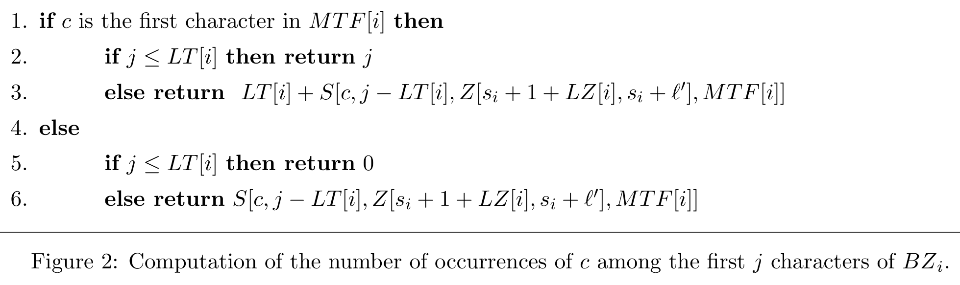
由于数组 LT 和 LZ 占用 O((u/ℓ) log ℓ) = O((u/log u) log log u) 比特,它们的引入不会改变过程 Occ 的渐近空间占用。
📄 原文
Since the arrays LT and LZ occupy O((u/ℓ) log ℓ) = O((u/log u) log log u) bits, their introduction does not change the asymptotic space occupancy of the procedure Occ.
📖 深入解析
为什么使用 1/2 编码?1/2 编码的核心性质是:每个编码位 bj 对应恰好 (bj + 1)·2j 个零。这意味着零串的编码可以在任意位边界处切分,而无需跨位协同。相比之下,若使用普通的二进制编码(如直接存储长度 m),切分编码将导致两个桶都无法正确解码。1/2 编码的这种「可切分性」使得我们可以在桶边界处自然地将编码 ε 分割为两部分,每部分都能独立解码出正确的零个数。这就是为什么在 FM-index 的 Run-Length Encoding 中必须选择 1/2 编码而非简单二进制编码的关键原因。
跨桶零串的巧妙记账:LT 和 LZ 两个数组的设计非常精巧。LT[i] 记录的是 BTmtfi 开头有多少个零未被 BZi 忠实编码(因为它们属于从上一个桶延续过来的零串),LZ[i] 则记录 BZi 中对应的偏移量。在实际查询时:若 j ≤ LT[i],则 BZi 的前 j 个位置全部对应于零(因为被检查字符 c 恰是 MTF[i] 的第一个字符——它在零串结束后才会首次出现);若 j > LT[i],则他跳到真正「忠实」的部分(j − LT[i]),再通过 LZ[i] 对齐 BZi 中的编码位置,然后调用表 S 进行常规查询。这个设计的精妙之处在于:它将跨桶边界的不完整零串问题转化为一个简单的偏移修正,而无需存储额外的零串信息。
算法伪代码的解读:图 2 中的算法分四种情况。情况 1-2(第 1-3 行):c 是 MTF[i] 列表中的第一个字符。这意味着在零串消除后,该桶的第一个非零字符才是 c。因此,在 LT[i] 位置之前的 j 个位置必然全是零(对应零串部分),直接返回 j;超出 LT[i] 的部分则跳到忠实编码区(偏移 LZ[i])后用 S 查询。情况 4-6(第 4-6 行):c 不是第一个字符,因此零串部分不会贡献 c 的出现,j ≤ LT[i] 时直接返回 0,否则同样跳到忠实编码区查询。注意这里的「c is the first character in MTF[i]」是相对于每个桶的本地 MTF 列表而言的。
空间开销为何可忽略:LT 和 LZ 每桶各占用 O(log ℓ) 比特,共有 u/ℓ 个桶。由 ℓ = Θ(log u) 可知总开销为 O((u/log u) log log u) 比特,这是 o(u) 的低阶项,不改变 Occ 的渐近空间占用。这体现了 FM-index 设计中的一个普遍原则:只要辅助数组的大小控制在 o(u) 级别,就不会影响整体的压缩界。
附录 D. 引理 2 的证明
令 T̄[1,v] 表示取自非恒定大小字母表 Λ 的字符串,并令 T̄bw = bwt(T̄)。对每个 j = 0, 1, ..., 2/ε,我们构造字符串 T̄bwj:对每个字符 κ ∈ Λ,从 T̄bw 中每 logjε v 个连续出现的 κ 中选取一个。此外,我们对 T̄bwj 中也会出现在下一个字符串 T̄bwj+1 中的字符进行逻辑标记。注意 T̄bw0 = T̄bw,且 T̄bwj 的长度为 Θ(v / logjε v)。
📄 原文
Let T̄[1,v] denote a string drawn from an alphabet Λ of non-constant size, and let T̄bw = bwt(T̄). For each j = 0, 1, ..., 2/ε, we construct the string T̄bwj by selecting from T̄bw one out of logjε v consecutive occurrences of κ, for every character κ ∈ Λ. Moreover, we logically mark the characters of T̄bwj which occur in the next string T̄bwj+1. Notice that T̄bw0 = T̄bw and that the length of T̄bwj is Θ(v / logjε v).
现在考虑一个改良的 move-to-front 过程,称为 mtf*,它通过记录一个字符自其上次出现以来所见的字符数来编码 T̄bw 中的字符。对 j = 0, 1, ..., 2/ε,令 T̄mtf*j = mtf*(T̄bwj)。我们存储字符串 T̄mtf*0, T̄mtf*1, ..., T̄mtf*2/ε,并对 T̄bw2/ε 中的字符,还保留其在原始变换文本 T̄bw 中 LF 映射的显式值。
📄 原文
Now consider a modified move-to-front procedure, called mtf*, that encodes a character in T̄bw by the number of characters seen since its previous occurrence. For j = 0, 1, ..., 2/ε, let T̄mtf*j = mtf*(T̄bwj). We store the strings T̄mtf*0, T̄mtf*1, ..., T̄mtf*2/ε and, for the characters in T̄bw2/ε, we also keep the explicit value of their LF-mapping in the original transformed text T̄bw.
计算字符 κ = T̄bw[s] 的 LF[s] 的高层思想是:利用数组 T̄mtf*j 以 Θ((2/ε) logε v) = Θ(logε v) 步跳跃到 κ 的一个出现,该出现也位于 T̄bw2/ε 中。对于这个出现,我们拥有显式的 LF 映射,从而可以轻松重建 LF[s]。更准确地,我们从 T̄bw0[s] 出发,依次移动到 T̄bw1, T̄bw2, ..., T̄bw2/ε,并如下更新一个计数器 v。令 T̄bwj[i] 为当前检查的字符(初始时 j = 0, i = s, v = 0);若该字符 κ 已被标记,则操作完成,v 保持不变;否则,我们利用 T̄mtf*j[i] 中编码的距离,移动到 T̄bwj 中前一个 κ 的出现,并将 logjε v 加到计数器 v 上。注意,我们实际上隐式地跳过了原始 T̄bw 中 logjε v 个字符 κ 的出现,因此在 v 中对它们进行了计数。现在我们已经到达一个被标记的字符 κ,因此可以移动到其在 T̄bwj+1 中的对应副本。经过 Θ(logε v) 次迭代后,我们到达 T̄bw2/ε 中 κ 的一个副本,其关于 T̄bw 的 LF 映射已知。于是,我们将该值与 v 相加,从而在总计 Θ(log2ε v) 时间内得到 LF[s]。
📄 原文
The high-level idea to compute LF[s] for a character κ = T̄bw[s] is to use the arrays T̄mtf*j's to jump, in Θ((2/ε) logε v) = Θ(logε v) steps, to an occurrence of κ which is also in T̄bw2/ε. For this occurrence we have the explicit LF-mapping and we can easily reconstruct LF[s]. More precisely, we start from T̄bw0[s] and we move to T̄bw1, T̄bw2, ..., T̄bw2/ε updating a counter v as follows. Let T̄bwj[i] be the currently examined character (initially j = 0, i = s and v = 0); if this character κ is marked then we are done and v remains unchanged; otherwise we move to the previous copy of κ in T̄bwj using the distance encoded in T̄mtf*j[i] and sum logjε v to the counter v. Note that we are indeed implicitly jumping logjε v occurrences of the character κ in the original T̄bw, and thus we account for them in v. We have now reached a marked character κ, thus we can move to its corresponding copy in T̄bwj+1. After Θ(logε v) iterations, we reach a copy of κ in T̄bw2/ε for which its LF-mapping over T̄bw is available. Consequently, we sum this value with v and thus obtain LF[s] in overall Θ(log2ε v) time.
注意,在上述方案中我们不需要数组 T̄bwj:我们只需要访问存储在 T̄mtf*0, T̄mtf*1, ..., T̄mtf*2/ε 中的值。这对于实现次线性空间界至关重要。令 bin(i) 表示 i + 1 的二进制表示(占用 1 + ⌊log(i + 1)⌋ 比特)。对每个 j = 0, 1, ..., 2/ε,我们构造以下三个数组:
📄 原文
Note that in the above scheme we do not need the arrays T̄bwj's: we only need to access the values stored in T̄mtf*0, T̄mtf*1, ..., T̄mtf*2/ε. This is crucial to achieve a sublinear space bound. Let bin(i) denote the binary representation of i + 1 (which takes 1 + ⌊log(i + 1)⌋ bits). We construct the following three arrays for each j = 0, 1, ..., 2/ε:
- Zj 是一个简洁编码 T̄mtf*j 的字符串,由连接 bin(T̄mtf*j[1]) bin(T̄mtf*j[2]) ... bin(T̄mtf*j[v/logjε v]) 组成;
- Wj 是一个长度为 |Zj| 的二进制数组,满足 Wj[i] = 1 当且仅当 Zj[i] 是 T̄mtf*j 中某个值编码的起始位位置;
- Nj 是一个长度为 |Zj| 的二进制数组,满足 Nj[i] = 1 当且仅当 Wj[i] = 1 且 T̄bwj 中对应字符也出现在 T̄bwj+1 中(因此被标记)。
📄 原文
- Zj is a string succinctly encoding T̄mtf*j and consisting of the concatenation bin(T̄mtf*j[1]) bin(T̄mtf*j[2]) ... bin(T̄mtf*j[v/logjε v]);
- Wj is a binary array of length |Zj| such that Wj[i] = 1 iff Zj[i] is the starting bit-position of the encoding of a value in T̄mtf*j;
- Nj is a binary array of length |Zj| such that Nj[i] = 1 iff Wj[i] = 1 and the corresponding character of T̄bwj occurs also in T̄bwj+1 (and thus it is marked).
利用文献 [22] 中描述的 rank 和 select 过程,并应用于上述数组,我们可以在 O(1) 时间内实现前述 LF[s] 计算的每一步。具体而言,给定 T̄mtf*j 中从位位置 i 开始的编码,我们可以通过访问 Nj[i] 来检查其是否对应于被标记的字符 κ。若确实如此,我们统计 T̄bwj+1 中在 κ 之前的字符数(通过对 Nj[1,i] 进行 rank),最后通过 Nj+1 上的 select 找到 κ 在 T̄mtf*j+1 中的编码位置。若 κ 未被标记,则在 O(1) 时间内解码 Zj 中从第 i 位开始的 T̄mtf*j 条目,然后通过数组 Wj 上的 rank 和 select 操作跳转到 T̄bwj 中前一个 κ 的出现。总之,每个操作耗时 O(1),这证明了引理 2 的时间界。
📄 原文
Using the procedures rank and select described in [22] and applied on the arrays above, we can implement each step of the computation of LF[s] described before in O(1) time. Namely, given an encoding of T̄mtf*j starting at bit position i, we can check if this corresponds to a marked character κ by accessing Nj[i]. If this is the case we count the number of characters of T̄bwj+1 preceding κ (via rank over Nj[1,i]) and finally find the position of the encoding of κ in T̄mtf*j+1 (via select on Nj+1). If κ is not marked, then we decode in O(1) time the entry of T̄mtf*j starting at the i-th bit of Zj and then jump to the previous occurrence of κ in T̄bwj via rank and select operations over array Wj. In summary, each of these operations takes O(1) time, and this proves the time bound of Lemma 2.
为证明空间界,我们首先观察到:为 T̄bw2/ε 中字符保留的显式 LF 映射所占用的空间为 O(v/log v) 比特(我们存储 O(v/log2 v) 个条目,每个 O(log v) 比特)。数组 Zj、Wj、Nj 以及 rank 和 select 操作的数据结构占用 O(|Z0| + |Z1| + ... + |Z2/ε|) 比特的存储,因此为 O(|Z0|) 比特。引理得证,因为由文献 [6, 19] 可导出关系 |Z0| = O(v(1 + Hk(T̄)) + |Λ|k+1 (log |Λ| + log v))。
📄 原文
To prove the space bound we first observe that the space occupancy induced by the explicit LF-mapping kept for the characters in T̄bw2/ε is O(v/log v) bits (we store O(v/log2 v) entries of O(log v) bits each). The arrays Zj's, Wj's, Nj's and the data structures for the rank and select operations take O(|Z0| + |Z1| + ... + |Z2/ε|) bits of storage, hence O(|Z0|) bits. The lemma follows since from [6, 19] we can derive the relation |Z0| = O(v(1 + Hk(T̄)) + |Λ|k+1 (log |Λ| + log v)).
📖 深入解析
层次子采样——类跳表的加速思想:引理 2 证明的核心是一个多层次的子采样方案,其思想与跳表(skip list)非常相似。在最低层 j = 0,我们保留完整的 BWT 变换 T̄bw;在第 j 层,我们对每个字符 κ,每隔 logjε v 个出现仅保留一个样本(即采样率为 1/logjε v)。这形成了一个几何递减的层次结构:每一层的大小递减因子为 logε v。总层数为 2/ε(常数),因此从底层跳跃到顶层(T̄bw2/ε,此时采样率已经极高,大小仅为 O(v / log2 v))只需常数层。关键是:在每一层内部,若当前字符未被标记(即未被采样到上一层),我们可以用 mtf* 编码的距离「跳」到同一层中前一个被标记的同字符出现——这正是跳表中「向前跳过多余元素」的经典操作。
mtf* 与 mtf 的本质区别:标准的 MTF(move-to-front)编码将一个字符编码为其在最近使用的字符列表中的排名(0 表示刚出现过的字符,较大的数表示很久未见的字符)。而 mtf* 则是按「距离上次出现」来编码:T̄mtf*j[i] 存储的是 T̄bwj 中当前字符距离其前一个同字符出现之间经过的字符数。这两种编码在不同场景下各有优势:mtf 适合局部性强的文本压缩;mtf* 则在这个证明中起到了关键作用,因为它编码的值恰好就是「从这个出现跳到前一个出现需要跳过的步数」,从而使得同一层内的跳跃可以在 O(1) 时间内完成。
rank/select 如何实现 O(1) 跳跃:三个位向量 Zj、Wj、Nj 的组合使用非常精妙。Zj 是主数据(存储 mtf* 编码的变长二进制表示),Wj 标记每个编码的起始位置(因为编码是变长的),Nj 在 Wj 的基础上进一步标记哪些字符被采样到了上一层。具体的操作链如下:(1) 通过 Nj[i] 检查当前字符是否为被标记(采样)的字符;(2) 若是,通过 Nj[1,i] 上的 rank 统计在它之前有多少个被标记的同字符,然后通过 Nj+1 上的 select 定位到上一层中的对应位置;(3) 若不是,则利用 Wj 上的 rank/select 跳转到同一层中前一个同字符的出现位置。所有操作均可在 O(1) 时间内完成,这是 Jacobson [22] 的 rank/select 数据结构的经典结果。
空间界的推导逻辑:空间分析的链条清晰:最顶层的显式 LF 映射仅需 O(v/log v) 比特(条目数 v/log2 v,每条 log v 比特)。所有层次的位向量总存储量为 O(|Z0| + |Z1| + ... + |Z2/ε|)。由于每一层的采样率等比递减,这个级数的和由首项 |Z0| 主导,为 O(|Z0|)。而 |Z0| 恰好是原始 T̄bw 的 mtf* 编码的总比特数,由文献 [6, 19] 可知,它被 k 阶经验熵 Hk(T̄) 所界。这样就完整地证明了:对于非恒定大小字母表上的字符串,LF 映射可以在 O(logε v) 时间内计算,同时空间占用保持为 O((Hk(T̄) + 1)·v) + o(v) 比特——这正是引理 2 的结论。