摘要
我们描述了一种块排序无损数据压缩算法及其实现,并在相同硬件上比较了该实现与广泛使用的数据压缩器的性能。
📄 原文
We describe a block-sorting, lossless data compression algorithm, and our implementation of that algorithm. We compare the performance of our implementation with widely available data compressors running on the same hardware.
该算法通过对输入文本块施加可逆变换来工作。该变换本身不压缩数据,而是重新排列数据,使其更容易用简单算法(如移至前端编码)进行压缩。
📄 原文
The algorithm works by applying a reversible transformation to a block of input text. The transformation does not itself compress the data, but reorders it to make it easy to compress with simple algorithms such as move-to-front coding.
我们的算法在速度上与基于 Lempel-Ziv 技术的算法相当,但获得的压缩率接近最佳的统计建模技术。输入块的大小必须足够大(几千字节)才能获得良好的压缩效果。
📄 原文
Our algorithm achieves speed comparable to algorithms based on the techniques of Lempel and Ziv, but obtains compression close to the best statistical modelling techniques. The size of the input block must be large (a few kilobytes) to achieve good compression.
📖 深入解析
BWT 的核心理念是「先变换再压缩」——它本身不是一个压缩算法,而是一种可逆的数据重排列预处理步骤。块排序(block-sorting)将字符按照上下文聚集在一起,使得同一字符在变换后的 L 列中彼此靠近。这种聚集效应使得后续简单的局部自适应压缩算法(如 MTF + Huffman)能够取得接近复杂统计建模的压缩率,同时保持 LZ 系列的速度优势。BWT 开创性地将「无损压缩」解耦为两个独立阶段:可逆变换(暴露冗余)和前端压缩(消除冗余)。这一思想后来成为 BWA 基因组比对工具及 FM-index 的基础。
1. 引言
最广泛使用的数据压缩算法基于 Lempel 和 Ziv 的序列数据压缩器 [1, 2]。统计建模技术可能产生更优的压缩效果 [3],但速度明显更慢。
📄 原文
The most widely used data compression algorithms are based on the sequential data compressors of Lempel and Ziv [1, 2]. Statistical modelling techniques may produce superior compression [3], but are significantly slower.
本文提出了一种技术,其压缩率与统计建模技术相差约一个百分点以内,但速度与基于 Lempel-Ziv 的算法相当。
📄 原文
In this paper, we present a technique that achieves compression within a percent or so of that achieved by statistical modelling techniques, but at speeds comparable to those of algorithms based on Lempel and Ziv's.
我们的算法不是按顺序处理输入,而是将文本块作为一个整体单位处理。其思想是:对文本块施加一个可逆变换,生成一个包含相同字符但更容易被简单压缩算法压缩的新块。这种变换倾向于将字符聚集在一起,使得找到某个字符靠近相同字符的另一个实例的概率显著增加。这类文本可以用快速局部自适应算法轻松压缩,例如移至前端编码 [4] 结合 Huffman 或算术编码。
📄 原文
Our algorithm does not process its input sequentially, but instead processes a block of text as a single unit. The idea is to apply a reversible transformation to a block of text to form a new block that contains the same characters, but is easier to compress by simple compression algorithms. The transformation tends to group characters together so that the probability of finding a character close to another instance of the same character is increased substantially. Text of this kind can easily be compressed with fast locally-adaptive algorithms, such as move-to-front coding [4] in combination with Huffman or arithmetic coding.
简言之,我们的算法通过以下方式变换一个包含 N 个字符的字符串 S:构造 S 的 N 个旋转(循环移位),按字典序对它们排序,然后提取每个旋转的最后一个字符。由这些字符构成字符串 L,其中 L 的第 i 个字符是第 i 个排序旋转的最后一个字符。除了 L 之外,算法还计算出原始字符串 S 在排序旋转列表中的索引 I。令人惊讶的是,仅凭 L 和 I 就存在一个高效的算法来恢复原始字符串 S。
📄 原文
Briefly, our algorithm transforms a string S of N characters by forming the N rotations (cyclic shifts) of S, sorting them lexicographically, and extracting the last character of each of the rotations. A string L is formed from these characters, where the ith character of L is the last character of the ith sorted rotation. In addition to L, the algorithm computes the index I of the original string S in the sorted list of rotations. Surprisingly, there is an efficient algorithm to compute the original string S given only L and I.
排序操作将具有相同起始字符的旋转聚集在一起。由于旋转的起始字符与末尾字符相邻,因此 L 中的连续字符在 S 中与相似的字符串相邻。如果字符的上下文是该字符的良好预测器,那么 L 将很容易通过简单的局部自适应压缩算法进行压缩。
📄 原文
The sorting operation brings together rotations with the same initial characters. Since the initial characters of the rotations are adjacent to the final characters, consecutive characters in L are adjacent to similar strings in S. If the context of a character is a good predictor for the character, L will be easy to compress with a simple locally-adaptive compression algorithm.
📖 深入解析
BWT 论文实际描绘了数据压缩的三条技术路线:(1)LZ 系列——基于滑动窗口/字典的序列压缩,速度最快但压缩率适中(代表:LZ77/LZ78 → LZW → gzip/deflate);(2)统计建模——基于概率上下文模型的压缩(如 PPM),压缩率最高但速度慢、内存开销大;(3)BWT 路线(块排序)——作为中间路线,先整块 BWT 变换再配合简单前端编码,速度接近 LZ、压缩率接近统计建模。BWT 的关键突破在于「块级别」而非「顺序」处理:通过对整个块排序所有循环移位,将每个字符的上下文信息编码进排列结构,使相同上下文的字符在 L 列中聚集,从而将全局上下文建模的高成本转化为一次性排序操作。这种设计后来意外地催生了 FM-index——在对上下文敏感的场景(如 DNA 序列比对)中,BWT 的重排特性使字符串匹配可以仅通过 L 和辅助数组高效完成,远超纯 LZ 或统计建模的应用边界。
2. 可逆变换
本节描述两个子算法。算法 C 执行压缩前对文本块施加的可逆变换,算法 D 执行逆操作。后续章节将介绍压缩变换块的方法。
📄 原文
This section describes two sub-algorithms. Algorithm C performs the reversible transformation that we apply to a block of text before compressing it, and Algorithm D performs the inverse operation. A later section suggests a method for compressing the transformed block of text.
在下文中,我们将字符串视为元素为字符的向量。
📄 原文
In the description below, we treat strings as vectors whose elements are characters.
2.1 算法 C:压缩变换(正向 BWT)
该算法的输入是一个由 N 个字符 S[0], …, S[N-1] 组成的字符串 S,这些字符选自有序字母表 X。为便于说明,我们给出一个运行示例:字符串 S = 'abraca',N = 6,字母表 X = {'a','b','c','r'}。
📄 原文
This algorithm takes as input a string S of N characters S[0]; …; S[N − 1] selected from an ordered alphabet X of characters. To illustrate the technique, we also give a running example, using the string S = 'abraca', N = 6, and the alphabet X = {'a','b','c','r'}.
C1. 排序旋转
构造一个概念上的 N×N 矩阵 M,其元素为字符,行是 S 的旋转(循环移位),并按字典序排序。矩阵 M 中至少有一行包含原始字符串 S。令 I 为第一个这样的行的索引(从 0 开始编号)。
📄 原文
C1. [sort rotations] Form a conceptual N × N matrix M whose elements are characters, and whose rows are the rotations (cyclic shifts) of S, sorted in lexicographical order. At least one of the rows of M contains the original string S. Let I be the index of the first such row, numbering from zero.
在我们的示例中,索引 I = 1,矩阵 M 为:
行 1: abraca
行 2: acaabr
行 3: bracaa
行 4: caabra
行 5: racaab
📄 原文
In our example, the index I = 1 and the matrix M is:
row 0: aabrac
row 1: abraca
row 2: acaabr
row 3: bracaa
row 4: caabra
row 5: racaab
C2. 找出旋转的最后一个字符
令字符串 L 为 M 的最后一列,其字符为 L[0], …, L[N-1](即 M[0,N-1], …, M[N-1,N-1])。变换的输出是 (L, I)。
📄 原文
C2. [find last characters of rotations] Let the string L be the last column of M, with characters L[0]; …; L[N − 1] (equal to M[0, N−1]; …; M[N−1, N−1]). The output of the transformation is the pair (L, I).
在我们的示例中,L = 'caraab',I = 1(来自步骤 C1)。
📄 原文
In our example, L = 'caraab' and I = 1 (from step C1).
2.2 算法 D:解压缩变换(逆 BWT)
我们使用算法 C 中介绍的示例和符号。算法 D 使用算法 C 的输出 (L, I) 重建其输入——长度为 N 的字符串 S。
📄 原文
We use the example and notation introduced in Algorithm C. Algorithm D uses the output (L, I) of Algorithm C to reconstruct its input, the string S of length N.
D1. 找出旋转的第一个字符
这一步计算算法 C 中矩阵 M 的第一列 F。通过对 L 中的字符排序得到 F。注意 M 的任何一列都是原始字符串 S 的一个排列,因此 L 和 F 都是 S 的排列,因而也是彼此的排列。此外,由于 M 的行已排序且 F 是 M 的第一列,F 中的字符也是排序的。
📄 原文
D1. [find first characters of rotations] This step calculates the first column F of the matrix M of Algorithm C. This is done by sorting the characters of L to form F. We observe that any column of the matrix M is a permutation of the original string S. Thus, L and F are both permutations of S, and therefore of one another. Furthermore, because the rows of M are sorted, and F is the first column of M, the characters in F are also sorted.
在我们的示例中,F = 'aaabcr'。
📄 原文
In our example, F = 'aaabcr'.
D2. 构建前驱字符列表
为便于解释,我们在矩阵 M 的内容上下文中描述此步骤。读者应记住,解压缩器无法获得完整的矩阵;此步骤仅需字符串 F、L 和索引 I(来自输入)。
📄 原文
To assist our explanation, we describe this step in terms of the contents of the matrix M. The reader should remember that the complete matrix is not available to the decompressor; only the strings F, L, and the index I (from the input) are needed by this step.
考虑矩阵 M 中以某个给定字符 ch 开头的行。算法 C 确保矩阵 M 的行按字典序排序,因此以 ch 开头的行按字典序排序。
📄 原文
Consider the rows of the matrix M that start with some given character ch. Algorithm C ensured that the rows of matrix M are sorted lexicographically, so the rows that start with ch are ordered lexicographically.
定义矩阵 M'——将 M 的每一行右移一个字符得到,即对每个 i = 0,…, N-1 和每个 j = 0,…, N-1,M'[i,j] = M[i, (j-1) mod N]。
📄 原文
We define the matrix M' formed by rotating each row of M one character to the right, so for each i = 0,…, N−1, and each j = 0,…, N−1, M'[i,j] = M[i, (j−1) mod N].
在我们的示例中,M 和 M' 为:
行 1: M = abraca M' = aabrac
行 2: M = acaabr M' = racaab
行 3: M = bracaa M' = abraca
行 4: M = caabra M' = acaabr
行 5: M = racaab M' = bracaa
📄 原文
In our example, M and M' are:
row 0: M = aabrac M' = caabra
row 1: M = abraca M' = aabrac
row 2: M = acaabr M' = racaab
row 3: M = bracaa M' = abraca
row 4: M = caabra M' = acaabr
row 5: M = racaab M' = bracaa
与 M 一样,M' 的每一行都是 S 的旋转,且 M 的每一行在 M' 中都有一个对应行。我们构造 M' 的方式使得 M' 的行按从第二个字符开始的字典序排序。因此,对于任意给定的字符 ch,M 中以 ch 开头的行与 M' 中以 ch 开头的行出现顺序相同。
📄 原文
Like M, each row of M' is a rotation of S, and for each row of M there is a corresponding row in M'. We constructed M' from M so that the rows of M' are sorted lexicographically starting with their second character. So, if we consider only those rows in M' that start with a character ch, they must appear in lexicographical order relative to one another; they have been sorted lexicographically starting with their second characters, and their first characters are all the same and so do not affect the sort order. Therefore, for any given character ch, the rows in M that begin with ch appear in the same order as the rows in M' that begin with ch.
在我们的示例中,这一点可以用于以 'a' 开头的行来验证。行 'aabrac'、'abraca' 和 'acaabr' 是 M 中的第 0、1、2 行,分别对应 M' 中的第 1、3、4 行。
📄 原文
In our example, this is demonstrated by the rows that begin with 'a'. The rows 'aabrac', 'abraca', and 'acaabr' are rows 0, 1, 2 in M and correspond to rows 1, 3, 4 in M'.
利用 F 和 L(M 和 M' 的第一列),我们计算向量 T,表示两个矩阵行之间的对应关系:对每个 j = 0,…, N-1,M' 的第 j 行对应于 M 的第 T[j] 行。
📄 原文
Using F and L, the first columns of M and M' respectively, we calculate a vector T that indicates the correspondence between the rows of the two matrices, in the sense that for each j = 0,…, N−1, row j of M' corresponds to row T[j] of M.
如果 L[j] 是 ch 在 L 中的第 k 次出现,则 T[j] = i,其中 F[i] 是 ch 在 F 中的第 k 次出现。注意 T 表示 F 元素与 L 元素之间的一一对应,且 F[T[j]] = L[j]。
📄 原文
If L[j] is the kth instance of ch in L, then T[j] = i where F[i] is the kth instance of ch in F. Note that T represents a one-to-one correspondence between elements of F and elements of L, and F[T[j]] = L[j].
在我们的示例中,T = (4 0 5 1 2 3)。
📄 原文
In our example, T is: (4 0 5 1 2 3).
D3. 输出 S
现在,对每个 i = 0,…, N-1,字符 L[i] 和 F[i] 是 M 第 i 行的最后一个和第一个字符。由于每一行都是 S 的一个旋转,字符 L[i] 在 S 中循环前于 F[i]。从 T 的构造可得 F[T[j]] = L[j]。代入 i = T[j] 得 L[T[j]] 在 S 中循环前于 L[j]。
📄 原文
Now, for each i = 0,…, N−1, the characters L[i] and F[i] are the last and first characters of the row i of M. Since each row is a rotation of S, the character L[i] cyclically precedes the character F[i] in S. From the construction of T, we have F[T[j]] = L[j]. Substituting i = T[j], we have L[T[j]] cyclically precedes L[j] in S.
索引 I 由算法 C 定义,使得 M 的第 I 行是 S。因此,S 的最后一个字符是 L[I]。我们使用向量 T 给出每个字符的前驱:对每个 i = 0,…, N-1:S[N-1-i] = L[Ti[I]],其中 T0[x] = x,且 Ti+1[x] = T[Ti[x]]。
📄 原文
The index I is defined by Algorithm C such that row I of M is S. Thus, the last character of S is L[I]. We use the vector T to give the predecessors of each character: for each i = 0,…, N−1: S[N−1−i] = L[Ti[I]], where T0[x] = x, and Ti+1[x] = T[Ti[x]].
这样就得到了原始输入字符串 S。
📄 原文
This yields S, the original input to the compressor.
在我们的示例中,S = 'abraca'。
📄 原文
In our example, S = 'abraca'.
我们本可以定义 T 使得字符串 S 从前向后生成,而非从后向前。上述描述与第 4.2 节中的伪代码一致。
📄 原文
We could have defined T so that the string S would be generated from front to back, rather than the other way around. The description above matches the pseudo-code given in Section 4.2.
序列 Ti[I](i = 0,…, N-1)不一定构成数字 0,…, N-1 的一个排列。如果原始字符串 S 的形式为 Zp(对于某个子串 Z 和某个 p > 1),那么序列 Ti[I] 也将为 Z'p 的形式(对于某个子序列 Z')。也就是说,S 中的重复将通过反复访问 T 的相同元素而生成。例如,如果 S = 'cancan',Z = 'can' 且 p = 2,那么序列 Ti[I] 将为 [2, 4, 0, 2, 4, 0]。
📄 原文
The sequence Ti[I] for i = 0,…, N−1 is not necessarily a permutation of the numbers 0,…, N−1. If the original string S is of the form Zp for some substring Z and some p > 1, then the sequence Ti[I] for i = 0,…, N−1 will also be of the form Z'p for some subsequence Z'. That is, the repetitions in S will be generated by visiting the same elements of T repeatedly. For example, if S = 'cancan', Z = 'can' and p = 2, the sequence Ti[I] for i = 0,…, N−1 will be [2, 4, 0, 2, 4, 0].
📖 解读:为什么行走序列会循环
这一段结论可以拆成三层来理解:
- T 本身永远是排列。F 列与 L 列都只是 S 的字符重排,同一字符「第 k 次出现」在两边一一对应、绝不冲突,所以 T 是 0,…,N-1 上的双射(bijection)。
- 排列 ≠ 走遍所有位置。任何排列都能分解成若干个互不相交的环(cycle)。从 I 出发反复应用 T,只能绕着 I 所在的那一个环转圈;只有当这个环恰好包含全部 N 个位置时,序列 Ti[I] 才是 0,…,N-1 的一个排列。
- 周期串把大环拆成小环。当 S = Zp(p > 1)时,S 的旋转出现重复(如 'cancan' 的第 0 个与第 3 个旋转都是 'cancan'),排序后矩阵出现相同行,T 随之裂成 p 个长度各为 |Z| 的环。行走于是只覆盖 |Z| 个不同位置,每个位置各被访问 p 次。
以 'cancan'(Z='can',p=2)为例:T = (2 3 4 5 0 1) 裂成 {2,4,0} 与 {1,3,5} 两个 3-环,I=2 落在 {2,4,0} 上,行走序列为 [2, 4, 0, 2, 4, 0]。逐个读出 L[i]:L[2]='n'、L[4]='a'、L[0]='c',即 'nac'2——因为 S 是从后向前重建的,这恰好是倒序的 S('cancan' 的倒序 = 'nac'2)。
反例 'abraca':T = (4 0 5 1 2 3) 只有一个 6-环,行走 1→0→4→2→5→3 覆盖全部 6 个位置各一次,序列 [1, 0, 4, 2, 5, 3] 才是 0,…,5 的排列。
一句话总结:整串的重复 ⟺ 行走位置序列的重复。逆变换的正确性并不依赖「走遍每个位置」——即使反复访问同一批位置,也照样能重建出 S。
📖 深入解析
一、LF-mapping 与向量 T 的关系
算法 D 中定义的向量 T 是现代 BWT 文献中「LF-mapping」(Last-to-First mapping)的早期形式。给定 L 和 F 两列,LF-mapping 将 L 中第 k 个出现的字符 ch 映射到 F 中第 k 个出现的相同字符 ch。向量 T[j] = i 即表示 L 中位置 j 的字符对应到 F 中位置 i 的同一个字符。T 的实质就是 LF-mapping 的向量表示。
二、算法 C / D 的数学本质
BWT 正向变换的数学本质可归纳为三步: (1) 构造所有循环移位(等价于在字符串末尾加终止符后的所有后缀,但有细微差别); (2) 按字典序排序这些旋转; (3) 提取排序矩阵的最后一列 L 和原始串的行号 I。
逆变换的本质是利用字典序排序带来的性质——同一字符在 F 和 L 中出现的相对顺序是相同的(因为对于以同一字符开头的行,其排序顺序取决于后续字符)。这一性质允许我们仅凭 L 和 I,通过 T 向量(LF-mapping)逐个恢复 S 中的字符。
三、T 向量构造算法(手工操作)
以 S = 'abraca' 为例:
- 步骤 1:将 L = 'caraab' 排序得 F = 'aaabcr'。
- 步骤 2:对每个字符 ch,建立「出现序号 → F 中位置」和「出现序号 → L 中位置」的映射。
- 示例(字符 'a'):F 中位置 0, 1, 2 分别是第 1, 2, 3 次出现;L 中位置 1, 3, 4 分别是第 1, 2, 3 次出现。
- 连边:对于 L 中每个位置 j,找到其对应字符 ch 的第 k 次出现,然后在 F 中找到第 k 次出现的位置 i,则 T[j] = i。
- 结果:T = (4 0 5 1 2 3):L[0]='c' → F[0+3]='c' → T[0]=4;L[1]='a'(第1次) → F[0]='a' → T[1]=0;L[2]='r' → F[5]='r' → T[2]=5;L[3]='a'(第2次) → F[1]='a' → T[3]=1;L[4]='a'(第3次) → F[2]='a' → T[4]=2;L[5]='b' → F[3]='b' → T[5]=3。
四、逆变换追踪(从后向前)
给定 L = 'caraab',I = 1,T = (4 0 5 1 2 3):
- S[5] = L[I] = L[1] = 'a'
- S[4] = L[T[I]] = L[T[1]] = L[0] = 'c'
- S[3] = L[T²[I]] = L[T[0]] = L[4] = 'a'
- S[2] = L[T³[I]] = L[T[4]] = L[2] = 'r'
- S[1] = L[T⁴[I]] = L[T[2]] = L[5] = 'b'
- S[0] = L[T⁵[I]] = L[T[3]] = L[1] = 'a'
得 S = 'abraca'。注意这是从后向前构建 S 的。
五、重复串的循环行走
序列 Ti[I] 不构成排列的原因、环分解的过程以及 'cancan' 的逐步行走,详见本段下方「解读」面板(内附图 2),此处不再重复。补充一点:这一观察对第 4 节高效实现中的分块解压缩策略很重要——行走会反复访问同一批位置,理解其环结构有助于正确设计与优化解压主循环(第 4.2 节伪代码中 i = P[i] + C[L[i]] 走的正是这条循环路径)。
六、与现代 BWT 的差异
现代 BWT 通常使用后缀数组(suffix array)实现,且通过添加唯一终止符 $ 来保证排序的确定性。论文的原始描述(1994 年)使用的是旋转矩阵 M 的全貌,这在概念上更直观但实现上不可行(需要 O(N²) 空间)。第 4 节将展示如何通过后缀排序将复杂度降至 O(N log N)。
七、BWT 的可逆性证明直觉
可逆性的关键在于:排序操作将同一上下文的旋转聚集在一起。F 列(排序后)和 L 列(排序后旋转的最后一个字符)通过「相同字符出现顺序保持一致」这一性质相互关联。这是一个非平凡的性质——正是它使得仅凭 L 和 I 即可唯一恢复原始字符串 S,无需存储完整的旋转矩阵。
3. 为什么变换后的字符串更易压缩
算法 C 对输入字符串 S 的旋转进行排序,生成由每个旋转的最后一个字符组成的字符串 L。
要理解为什么这有助于压缩,考虑一段英文文本中一个常见单词中的单个字母。以 'the' 中的字母 't' 为例,假设输入字符串包含许多 'the' 实例。
当输入的旋转列表被排序后,所有以 "he " 开头的旋转都排在一起;它们中很大一部分很可能以 't' 结尾。因此,L 串的一个区域将包含异常大量的 't' 字符,夹杂着在英语中可以出现在 "he " 之前的其他字符,如空格、's'、'T' 和 'S'。
同样的论点可应用于所有单词中的所有字符,因此 L 串的任何局部区域都可能包含大量的少数几个不同的字符。总体效果是,如果字符 ch 在 L 中靠近某点出现,那么它在同一附近再次出现的概率非常高,否则很低。
这种性质正是移至前端编码器 [4] 所需要的——它将一个字符 ch 的实例编码为自上一个 ch 出现以来所看到的不同字符的计数。应用到 L 串时,移至前端编码器的输出将以小数字为主,可以被高效的熵编码器进一步压缩。
📄 原文
Algorithm C sorts the rotations of an input string S, and generates the string L consisting of the last character of each rotation.
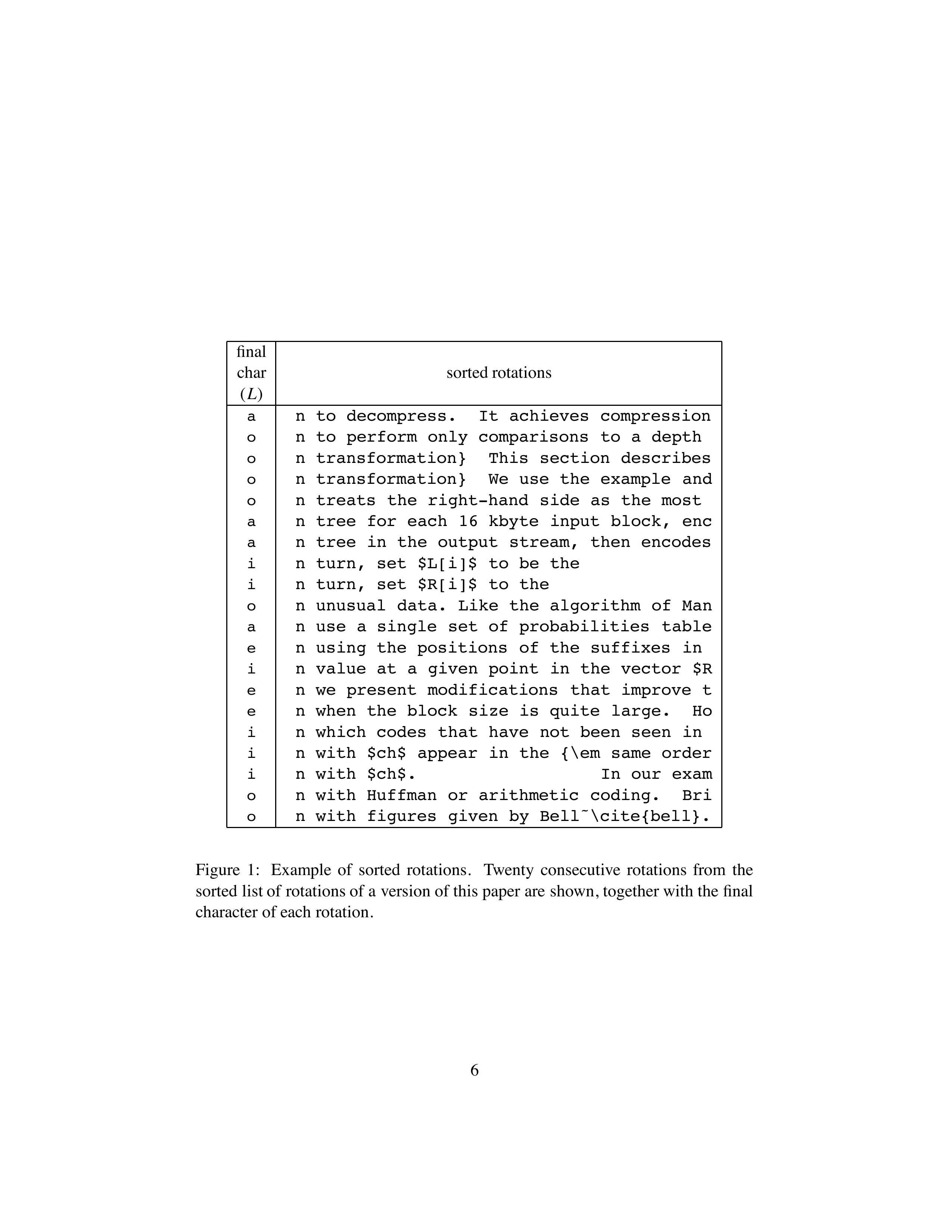
To see why this might lead to effective compression, consider the effect on a single letter in a common word in a block of English text. We will use the example of the letter 't' in the word 'the', and assume an input string containing many instances of 'the'.
When the list of rotations of the input is sorted, all the rotations starting with 'he ' will sort together; a large proportion of them are likely to end in 't'. One region of the string L will therefore contain a disproportionately large number of 't' characters, intermingled with other characters that can precede 'he ' in English, such as space, 's', 'T', and 'S'.
The same argument can be applied to all characters in all words, so any localized region of the string L is likely to contain a large number of a few distinct characters. The overall effect is that the probability that given character ch will occur at a given point in L is very high if ch occurs near that point in L, and is low otherwise.
This property is exactly the one needed for effective compression by a move-to-front coder [4], which encodes an instance of character ch by the count of distinct characters seen since the next previous occurrence of ch. When applied to the string L, the output of a move-to-front coder will be dominated by low numbers, which can be efficiently compressed by an entropy coder.
📖 深入解析
BWT 的核心效应是让字母根据"上下文"聚集。以 'the' 为例:
- 在一个句子 "I have the book. I see the cat." 中,'the' 出现了两次。BWT 把以 "he " 开头的旋转排在一起——这些旋转的最后一个字符恰好是 't'(因为 'the' 中 't' 在 "he" 之前)。于是 L 串中 't' 会成片出现。
- 这种聚集效应的数学本质是:排序使得具有相同前缀的行聚在一起,而前缀正是紧邻最后一个字符右侧的上下文。因此 L 中相邻字符在原始文本中共享相似的右侧上下文,这种"上下文局部性"使得 L 中相同字符倾向于聚集。
聚集效应带来两种对压缩有益的性质:
- 短程相关性:同一字符出现的间隔很短。MTF 编码会把"刚见过的字符"编码为小数字(0, 1, 2...),而小数字占用的熵更少。
- 局部字母表收缩:在 L 的任意局部区域,实际出现的不同字符种类远少于全局字母表。这降低了 MTF 输出的最大数值,也降低了 Huffman/算术编码的模型复杂度。
这种"先变换后压缩"的思路在当时很新颖,后来人们发现 BWT 不仅能帮压缩,还能做索引(FM-index),那才是它在生物信息学领域大放异彩的开始。
为完整起见,我们现在给出编码算法 C 输出的一种可行方法及其逆运算的细节。将编码与解码操作分别与算法 C 和 D 组合,即可构成一个完整的压缩算法。
📄 原文
For completeness, we now give details of one possible way to encode the output of Algorithm C, and the corresponding inverse operation. A complete compression algorithm is created by combining these encoding and decoding operations with Algorithms C and D.
算法 M:移至前端编码(MTF)
该算法对算法 C 的输出 (L, I) 进行编码,其中 L 是长度为 N 的字符串,I 是一个索引。它使用移至前端算法和 Huffman 或算术编码器对 L 进行编码。这里继续沿用算法 C 的运行示例。
📄 原文
Algorithm M: Move-to-front coding
This algorithm encodes the output (L, I) of Algorithm C, where L is a string of length N and I is an index. It encodes L using a move-to-front algorithm and a Huffman or arithmetic coder. The running example of Algorithm C is continued here.
M1. [移至前端编码] 该步骤通过对各个字符应用移至前端技术,对 L 中的每个字符进行编码。我们定义一个整数向量 R[0]; …; R[N−1],它们是字符 L[0]; …; L[N−1] 的编码。
📄 原文
M1. [move-to-front coding] This step encodes each of the characters in L by applying the move-to-front technique to the individual characters. We define a vector of integers R[0]; …; R[N−1], which are the codes for the characters L[0]; …; L[N−1].
初始化一个列表 Y,使其恰好包含字母表 X 中的每个字符一次。对于每个 i = 0,…, N−1,依次将 R[i] 设为字符 L[i] 在列表 Y 中前面的字符个数,然后将字符 L[i] 移至 Y 的前端。
📄 原文
Initialize a list Y of characters to contain each character in the alphabet X exactly once. For each i = 0,…, N−1 in turn, set R[i] to the number of characters preceding character L[i] in the list Y, then move character L[i] to the front of Y.
初始时取 Y = ['a','b','c','r'],L = 'caraab',我们计算出向量 R:(2, 1, 3, 1, 0, 3)。
📄 原文
Taking Y = ['a','b','c','r'] initially, and L = 'caraab', we compute the vector R: (2, 1, 3, 1, 0, 3).
M2. [编码] 对 R 的每个元素应用 Huffman 或算术编码,将每个元素视为一个独立的待编码标记。只要解压器能够执行逆操作,任何编码技术都可以使用。将此编码过程的输出记为 OUT。算法 C 的输出是 (OUT, I),其中 I 是在步骤 C1 中计算出的值。
📄 原文
M2. [encode] Apply Huffman or arithmetic coding to the elements of R, treating each element as a separate token to be coded. Any coding technique can be applied as long as the decompressor can perform the inverse operation. Call the output of this coding process OUT. The output of Algorithm C is the pair (OUT, I) where I is the value computed in step C1.
算法 W:移至前端解码
该算法是算法 M 的逆过程。它从 (OUT, I) 计算出 (L, I)。我们假设步骤 M1 中使用的列表 Y 的初始值对解压器可用,且步骤 M2 中使用的编码方案具有逆操作。
📄 原文
Algorithm W: Move-to-front decoding
This algorithm is the inverse of Algorithm M. It computes the pair (L, I) from the pair (OUT, I). We assume that the initial value of the list Y used in step M1 is available to the decompressor, and that the coding scheme used in step M2 has an inverse operation.
W1. [解码] 使用步骤 M2 中所用编码方案的逆操作对编码流 OUT 进行解码,结果是一个由 N 个整数组成的向量 R。在我们的示例中,R 为:(2, 1, 3, 1, 0, 3)。
📄 原文
W1. [decode] Decode the coded stream OUT using the inverse of the coding scheme used in step M2. The result is a vector R of N integers. In our example, R is: (2, 1, 3, 1, 0, 3).
W2. [逆移至前端编码] 本步骤的目标是:给定移至前端编码 R[0]; …; R[N−1],计算长度为 N 的字符串 L。初始化一个列表 Y,使其按与步骤 M1 相同的顺序包含字母表 X 中的字符。对于每个 i = 0,…, N−1,依次将 L[i] 设为列表 Y 中位置 R[i] 处的字符(从 0 编号),然后将该字符移至 Y 的前端。
📄 原文
W2. [inverse move-to-front coding] The goal of this step is to calculate a string L of N characters, given the move-to-front codes R[0]; …; R[N−1]. Initialize a list Y of characters to contain the characters of the alphabet X in the same order as in step M1. For each i = 0,…, N−1 in turn, set L[i] to be the character at position R[i] in list Y (numbering from 0), then move that character to the front of Y.
得到的字符串 L 是算法 C 中矩阵 M 的最后一列。该算法的输出是 (L, I),即算法 D 的输入。初始时取 Y = ['a','b','c','r'](与算法 M 相同),我们计算出字符串 L = 'caraab'。
📄 原文
The resulting string L is the last column of matrix M of Algorithm C. The output of this algorithm is the pair (L, I), which is the input to Algorithm D. Taking Y = ['a','b','c','r'] initially (as in Algorithm M), we compute the string L = 'caraab'.
📖 深入解析
MTF 编码的思路很直观:刚用过的字符很可能马上再用。把它放在列表最前面,下次编码时只需要小数字。
MTF 为什么配合 BWT 特别有效?BWT 之后,L 串中相同字符倾向于聚集。想象 L = "aaabcr"(3 个 'a' 连在一起):
- 第一个 'a':在列表 ['a','b','c','r'] 中位置 0 → 输出 0,然后将 'a' 移到最前 → ['a','b','c','r'](不变)
- 第二个 'a':位置 0 → 输出 0
- 第三个 'a':位置 0 → 输出 0
连续三个 'a' 编码为 0, 0, 0——可以在 Huffman 中用极少的比特表示。更一般地,当 L 中连续出现相同字符时,MTF 输出连续为 0,形成 0 游程。小数字占用的熵极少,而 0 游程还可以用游程编码进一步压缩。
但如果字符分散在各处(没做 BWT 的原始文本),MTF 会输出许多大数字,压缩效果很差。所以 BWT + MTF 是天生一对。
4. 高效实现
移至前端、Huffman 和算术编码的高效实现已广为人知。这里我们集中讨论算法 C 和 D 中不寻常的步骤。
📄 原文
Efficient implementations of move-to-front, Huffman, and arithmetic coding are well known. Here we concentrate on the unusual steps in Algorithms C and D.
4.1 压缩
压缩速度最重要的因素是排序输入块旋转所需的时间。直接应用快速排序所需额外空间很小(每个字符一个词),在大多数输入数据上表现也不错。然而,其最坏情况性能较差。
📄 原文
The most important factor in compression speed is the time taken to sort the rotations of the input block. A simple application of quicksort requires little additional space (one word per character), and works fairly well on most input data. However, its worst-case performance is poor.
实现算法 C 的一种更快方式,是把排序旋转的问题归约为对某个相关字符串的后缀进行排序的问题。
📄 原文
A faster way to implement Algorithm C is to reduce the problem of sorting the rotations to the problem of sorting the suffixes of a related string.
要压缩字符串 S,先构造字符串 S',它是 S 与 EOF(一个不在 S 中出现的新字符)的拼接。然后对 S' 应用算法 C。由于 EOF 不同于 S' 中的所有其他字符,S' 的后缀的排序顺序与 S' 的旋转的排序顺序相同。因此,要排序旋转,只需排序 S' 的后缀即可。这可以通过构建后缀树在线性时间和空间内完成,之后按字典序遍历该树即可恢复排序后的后缀。我们在一个算法 C 的实现中使用了 McCreight 的后缀树构造算法 [5]。在处理文本文件时,它的性能在已知最快技术的 40% 以内。遗憾的是,后缀树算法每个输入字符需要超过四个机器字的存储空间。
📄 原文
To compress a string S, first form the string S', which is the concatenation of S with EOF, a new character that does not appear in S. Now apply Algorithm C to S'. Because EOF is different from all other characters in S', the suffixes of S' sort in the same order as the rotations of S'. Hence, to sort the rotations, it suffices to sort the suffixes of S'. This can be done in linear time and space by building a suffix tree, which then can be walked in lexicographical order to recover the sorted suffixes. We used McCreight's suffix tree construction algorithm [5] in an implementation of Algorithm C. Its performance is within 40% of the fastest technique we have found when operating on text files. Unfortunately, suffix tree algorithms need space for more than four machine words per input character.
Manber 和 Myers 给出了一个在 O(N log N) 时间内排序字符串后缀的简单算法 [6]。他们所描述的算法每个输入字符只需两个字的存储空间。该算法的工作原理是:先按后缀的前 i 个字符排序,然后将后缀在已排序数组中的位置作为排序关键字,再进行一次基于前 2i 个字符的排序。遗憾的是,他们算法的性能明显差于后缀树方法。
📄 原文
Manber and Myers give a simple algorithm for sorting the suffixes of a string in O(N log N) time [6]. The algorithm they describe requires only two words per input character. The algorithm works by sorting suffixes on their first i characters, then using the positions of the suffixes in the sorted array as the sort key for another sort on the first 2i characters. Unfortunately, the performance of their algorithm is significantly worse than the suffix tree approach.
到目前为止,我们尝试过的最快方案使用快速排序的一种变体来生成排序后的后缀列表。在处理文本时,其性能显著优于后缀树,且使用的空间少得多。但与后缀树不同的是,在处理某些类型的数据时,其性能可能大幅退化。与 Manber 和 Myers 的算法一样,我们的算法每个输入字符只使用两个字的存储空间。
📄 原文
The fastest scheme we have tried so far uses a variant of quicksort to generate the sorted list of suffixes. Its performance is significantly better than the suffix tree when operating on text, and it uses significantly less space. Unlike the suffix tree however, its performance can degrade considerably when operating on some types of data. Like the algorithm of Manber and Myers, our algorithm uses only two words per input character.
算法 Q:后缀快速排序
该算法对字符串 S 的后缀进行排序,S 包含 N 个字符 S[0; …; N−1]。算法对 S 的后缀应用快速排序的修改版本。我们首先给出算法的简单版本,然后给出提高速度并降低糟糕性能发生可能性的修改。
📄 原文
This algorithm sorts the suffixes of the string S, which contains N characters S[0; …; N−1]. The algorithm works by applying a modified version of quicksort to the suffixes of S. First we present a simple version of the algorithm. Then we present modifications that improve the speed and make bad performance less likely.
Q1. [构造扩展字符串] 设 k 为能放入一个机器字的字符个数。构造字符串 S',即向 S 追加 k 个额外的 EOF 字符(EOF 不在 S 中出现)。
📄 原文
Q1. [form extended string] Let k be the number of characters that fit in a machine word. Form the string S' from S by appending k additional EOF characters to S, where EOF does not appear in S.
Q2. [构造字数组] 初始化一个由 N 个字组成的数组 W,W[0; …; N−1],使得 W[i] 包含字符 S'[i; …; i+k−1],且排列方式使字上的整数比较与这 k 个字符构成的字符串上的字典序比较一致。将字符打包进字有两个好处:允许在比较两个前缀时用对齐的内存访问一次比较 k 个字节;并且可以消除许多慢速情况(见步骤 Q7)。
📄 原文
Q2. [form array of words] Initialize an array W of N words W[0; …; N−1], such that W[i] contains the characters S'[i; …; i+k−1] arranged so that integer comparisons on the words agree with lexicographic comparisons on the k-character strings. Packing characters into words has two benefits: It allows two prefixes to be compared k bytes at a time using aligned memory accesses, and it allows many slow cases to be eliminated (described in step Q7).
Q3. [构造后缀数组] 本步骤初始化一个由 N 个整数组成的数组 V。如果 V 的某个元素为 j,它表示以 S'[j] 为第一个字符的 S' 的后缀。算法完成后,后缀 V[i] 将按字典序排列,成为第 i 个后缀。初始化整数数组 V,使得对每个 i = 0,…, N−1:V[i] = i。
📄 原文
Q3. [form array of suffixes] In this step we initialize an array V of N integers. If an element of V contains j, it represents the suffix of S' whose first character is S'[j]. When the algorithm is complete, suffix V[i] will be the ith suffix in lexicographical order. Initialize an array V of integers so that for each i = 0,…, N−1: V[i] = i.
Q4. [基数排序] 以每个后缀的前两个字符为排序关键字,对 V 的元素进行排序。这可以用基数排序高效完成。
📄 原文
Q4. [radix sort] Sort the elements of V, using the first two characters of each suffix as the sort key. This can be done efficiently using radix sort.
Q5. [遍历字母表中的每个字符] 对字母表中的每个字符 ch,执行步骤 Q6、Q7。当这次遍历完成时,V 就表示 S 的已排序后缀,算法终止。
📄 原文
Q5. [iterate over each character in the alphabet] For each character ch in the alphabet, perform steps Q6, Q7. Once this iteration is complete, V represents the sorted suffixes of S, and the algorithm terminates.
Q6. [对以 ch 开头的后缀进行快速排序] 对字母表中的每个字符 ch':对 V 中以 ch 后跟 ch' 开头的元素应用快速排序。在快速排序的实现中,通过索引数组 W 来比较 V 的元素所代表的后缀。在每次递归步骤中,记录组内已比较相等的字符个数,使它们无需再比较。
📄 原文
Q6. [quicksort suffixes starting with ch] For each character ch' in the alphabet: Apply quicksort to the elements of V starting with ch followed by ch'. In the implementation of quicksort, compare the elements of V by comparing the suffixes they represent by indexing into the array W. At each recursion step, keep track of the number of characters that have compared equal in the group, so that they need not be compared again.
现在,所有以 ch 开头的后缀都已排入 V 中的最终位置。
📄 原文
All the suffixes starting with ch have now been sorted into their final positions in V.
Q7. [更新排序关键字] 对 V[i] 中每个对应于以 ch 开头的后缀(即满足 S[V[i]] = ch)的元素,将 W[V[i]] 设为一个其高位包含 ch(与之前相同)、低位包含 i 的值(步骤 Q2 将其设为初始 ch 之后的 k−1 个字符)。W[V[i]] 的新值与旧值排序位置相同,但它有一个理想的特性:与 W 中所有其他值都不同。这加速了后续的排序操作,因为与新元素的比较不可能相等。
📄 原文
Q7. [update sort keys] For each element V[i] corresponding to a suffix starting with ch (that is, for which S[V[i]] = ch), set W[V[i]] to a value with ch in its high-order bits (as before) and with i in its low-order bits (which step Q2 set to the k−1 characters following the initial ch). The new value of W[V[i]] sorts into the same position as the old value, but has the desirable property that it is distinct from all other values in W. This speeds up subsequent sorting operations, since comparisons with the new elements cannot compare equal.
这个基本算法可以在许多方面进行改进。一个明显的改进是:在步骤 Q5 中,从 S 中最不常见的字符开始依次选择字符 ch,直到最常见的字符。这使步骤 Q7 的更新产生最大效果。
📄 原文
This basic algorithm can be refined in a number of ways. An obvious improvement is to pick the character ch in step Q5 starting with the least common character in S, and proceeding to the most common. This allows the updates of step Q7 to have the greatest effect.
如上所述,当 S 包含许多重复子串时,该算法表现不佳。我们用两种机制处理这个问题。第一种机制处理单一重复字符构成的字符串,即用以下步骤替换步骤 Q6。
📄 原文
As described, the algorithm performs poorly when S contains many repeated substrings. We deal with this problem with two mechanisms. The first mechanism handles strings of a single repeated character by replacing step Q6 with the following steps.
Q6a. [对以 ch; ch'(ch ≠ ch')开头的后缀进行快速排序] 对字母表中每个 ch' ≠ ch 的字符:对 V 中以 ch 后跟 ch' 开头的元素应用快速排序。在快速排序的实现中,通过索引数组 W 比较 V 的元素所代表的后缀。在每次递归步骤中,记录组内已比较相等的字符个数,使它们无需再比较。
📄 原文
Q6a. [quicksort suffixes starting ch; ch' where ch ≠ ch'] For each character ch' ≠ ch in the alphabet: Apply quicksort to the elements of V starting with ch followed by ch'. In the implementation of quicksort, compare the elements of V by comparing the suffixes they represent by indexing into the array W. At each recursion step, keep track of the number of characters that have compared equal in the group, so that they need not be compared again.
Q6b. [对以 ch; ch 开头的低位后缀排序] 本步骤对以 ch 开头、排序时位于无限 ch 字符序列之前的长游程后缀进行排序。我们观察到:在这类后缀中,以 ch 开头的前缀较长者排在较短者之后,长度相等时按游程末尾字符的顺序排序。这个顺序可以用一个从最短后缀开始的简单循环得到。
📄 原文
Q6b. [sort low suffixes starting ch; ch] This step sorts the suffixes starting runs which would sort before an infinite string of ch characters. We observe that among such suffixes, long initial runs of character ch sort after shorter initial runs, and runs of equal length sort in the same order as the characters at the ends of the run. This ordering can be obtained with a simple loop over the suffixes, starting with the shortest.
设 V[i] 表示以 ch 开头的字典序最小的后缀。设 j 为满足后缀 V[j] 以 ch; ch 开头的最小值。
📄 原文
Let V[i] represent the lexicographically least suffix starting with ch. Let j be the lowest value such that suffix V[j] starts with ch; ch.
while not (i = j) do
  if (V[i] > 0) and (S[V[i]-1] = ch) then
    V[j] := V[i]-1;
    j := j + 1
  end;
  i := i + 1
end;
现在,所有以 ch; ch 开头、且字典序小于无限 ch 字符序列的后缀都已排序。
📄 原文
All the suffixes that start with ch; ch and that are lexicographically less than an infinite sequence of ch characters are now sorted.
Q6c. [对以 ch; ch 开头的高位后缀排序] 本步骤对以 ch 开头、排序时位于无限 ch 字符序列之后的长游程后缀进行排序。此步骤与 Q6b 非常相似,只是循环方向相反。设 V[i] 表示以 ch 开头的字典序最大的后缀。设 j 为满足后缀 V[j] 以 ch; ch 开头的最大值。
📄 原文
Q6c. [sort high suffixes starting ch; ch] This step sorts the suffixes starting runs which would sort after an infinite string of ch characters. This step is very like step Q6b, but with the direction of the loop reversed. Let V[i] represent the lexicographically greatest suffix starting with ch. Let j be the highest value such that suffix V[j] starts with ch; ch.
while not (i = j) do
  if (V[i] > 0) and (S[V[i]-1] = ch) then
    V[j] := V[i]-1;
    j := j - 1
  end;
  i := i - 1
end;
现在,所有以 ch; ch 开头、且字典序大于无限 ch 字符序列的后缀都已排序。
📄 原文
All the suffixes that start with ch; ch and that are lexicographically greater than an infinite sequence of ch characters are now sorted.
第二种机制处理由多个字符构成的重复子串的长字符串。对这类字符串,我们使用与 Manber 和 Myers 方案类似的倍增技术。我们将快速排序实现限制为只比较到深度 D。在 V 的对应元素中用一位记录后缀尚未排序的位置。
📄 原文
The second mechanism handles long strings of a repeated substring of more than one character. For such strings, we use a doubling technique similar to that used in Manber and Myers' scheme. We limit our quicksort implementation to perform comparisons only to a depth D. We record where suffixes have been left unsorted with a bit in the corresponding elements of V.
一旦步骤 Q1 到 Q7 完成,数组 W 的元素就指示了排到 D × k 个字符的位置,因为每次比较都比较 k 个字符。如果 V 中仍有未排序的部分,我们只需再次排序,限制比较深度仍为 D。这一次,每次比较比较 D × k 个字符,得到按前 D² × k 个字符排序的后缀列表。我们重复这一过程,直到整个字符串排序完成。
📄 原文
Once steps Q1 to Q7 are complete, the elements of the array W indicate sorted positions up to D × k characters, since each comparison compares k characters. If unsorted portions of V remain, we simply sort them again, limiting the comparison depth to D as before. This time, each comparison compares D × k characters, to yield a list of suffixes sorted on their first D² × k characters. We repeat this process until the entire string is sorted.
基数排序、精心实现的快速排序以及处理重复字符串的机制相结合,产生了一种在大多数输入上极快的排序算法,而且在真实输入数据上表现很差的概率极低。
📄 原文
The combination of radix sort, a careful implementation of quicksort, and the mechanisms for dealing with repeated strings produce a sorting algorithm that is extremely fast on most inputs, and is quite unlikely to perform very badly on real input data.
我们目前正在研究快速排序的更多变体。以下方法看起来很有前景。通过把 Q6a–Q6c 的技术应用于所有重叠的重复字符串,并在哈希表中缓存先前计算出的排序结果,我们可以得到一个与修改后的算法 Q 用时大致相同的后缀排序算法,但每个输入字符只需 6 个字节的空间(4 字节存指针,1 字节存输入字符本身,1 字节为哈希表中均摊的空间)。该方法在最坏情况下性能较差,但糟糕情况在实践中似乎很少见。
📄 原文
We are currently investigating further variations of quicksort. The following approach seems promising. By applying the technique of Q6a–Q6c to all overlapping repeated strings, and by caching previously computed sort orders in a hash table, we can produce an algorithm that sorts the suffixes of a string in approximately the same time as the modified algorithm Q, but using only 6 bytes of space per input character (4 bytes for a pointer, 1 byte for the input character itself, and 1 byte amortized space in the hash table). This approach has poor performance in the worst case, but bad cases seem to be rare in practice.
4.2 解压缩
步骤 D1 和 D2 可以高效地仅通过两趟数据扫描和一趟字母表扫描完成,如下面的伪代码所示。第一趟扫描中,我们构造两个数组:C[alphabet] 和 P[0; …; N−1]。C[ch] 是 L 中所有在字母表顺序上位于字符 ch 之前的字符的实例总数。P[i] 是字符 L[i] 在 L 的前缀 L[0; …; i−1] 中出现的次数。实践中,这第一趟扫描可以与移至前端解码步骤合并。给定数组 L、C、P,步骤 D2 中定义的数组 T 为:对每个 i = 0,…, N−1:T[i] = P[i] + C[L[i]]
📄 原文
Steps D1 and D2 can be accomplished efficiently with only two passes over the data, and one pass over the alphabet, as shown in the pseudo-code below. In the first pass, we construct two arrays: C[alphabet] and P[0; …; N−1]. C[ch] is the total number of instances in L of characters preceding character ch in the alphabet. P[i] is the number of instances of character L[i] in the prefix L[0; …; i−1] of L. In practice, this first pass could be combined with the move-to-front decoding step. Given the arrays L, C, P, the array T defined in step D2 is given by:
第二趟数据扫描中,我们使用起始位置 I 完成算法 D 以生成 S。初始时,C 的所有元素为零,矩阵 M 的最后一列是向量 L[0; …; N−1]。
📄 原文
In a second pass over the data, we use the starting position I to complete Algorithm D to generate S. Initially, all elements of C are zero, and the last column of matrix M is the vector L[0; …; N−1].
for i := 0 to N-1 do
  P[i] := C[L[i]];
  C[L[i]] := C[L[i]] + 1
end;
现在 C[ch] 是 L 中字符 ch 的实例个数。P[i] 是字符 L[i] 在 L 的前缀 L[0; …; i−1] 中出现的次数。

sum := 0;
for ch := FIRST(alphabet) to LAST(alphabet) do
  sum := sum + C[ch];
  C[ch] := sum - C[ch];
end;
现在 C[ch] 是 L 中所有在字母表顺序上位于 ch 之前的字符的实例总数。

i := I;
for j := N-1 downto 0 do
  S[j] := L[i];
  i := P[i] + C[L[i]]
end
解压结果即 S[0; …; N−1]。
📄 原文
The decompressed result is now S[0; …; N−1].
📄 原文(4.1 与 4.2 完整原文)
4.1 Compression
The most important factor in compression speed is the time taken to sort the rotations of the input block. A simple application of quicksort requires little additional space (one word per character), and works fairly well on most input data. However, its worst-case performance is poor.
A faster way to implement Algorithm C is to reduce the problem of sorting the rotations to the problem of sorting the suffixes of a related string.
To compress a string S, first form the string S', which is the concatenation of S with EOF, a new character that does not appear in S. Now apply Algorithm C to S'. Because EOF is different from all other characters in S', the suffixes of S' sort in the same order as the rotations of S'. Hence, to sort the rotations, it suffices to sort the suffixes of S'. This can be done in linear time and space by building a suffix tree, which then can be walked in lexicographical order to recover the sorted suffixes. We used McCreight's suffix tree construction algorithm [5] in an implementation of Algorithm C. Its performance is within 40% of the fastest technique we have found when operating on text files. Unfortunately, suffix tree algorithms need space for more than four machine words per input character.
Manber and Myers give a simple algorithm for sorting the suffixes of a string in O(N log N) time [6]. The algorithm they describe requires only two words per input character. The algorithm works by sorting suffixes on their first i characters, then using the positions of the suffixes in the sorted array as the sort key for another sort on the first 2i characters. Unfortunately, the performance of their algorithm is significantly worse than the suffix tree approach.
The fastest scheme we have tried so far uses a variant of quicksort to generate the sorted list of suffixes. Its performance is significantly better than the suffix tree when operating on text, and it uses significantly less space. Unlike the suffix tree however, its performance can degrade considerably when operating on some types of data. Like the algorithm of Manber and Myers, our algorithm uses only two words per input character.
Algorithm Q: Fast quicksorting on suffixes
This algorithm sorts the suffixes of the string S, which contains N characters S[0; …; N−1]. The algorithm works by applying a modified version of quicksort to the suffixes of S. First we present a simple version of the algorithm. Then we present modifications that improve the speed and make bad performance less likely.
Q1. [form extended string] Let k be the number of characters that fit in a machine word. Form the string S' from S by appending k additional EOF characters to S, where EOF does not appear in S.
Q2. [form array of words] Initialize an array W of N words W[0; …; N−1], such that W[i] contains the characters S'[i; …; i+k−1] arranged so that integer comparisons on the words agree with lexicographic comparisons on the k-character strings. Packing characters into words has two benefits: It allows two prefixes to be compared k bytes at a time using aligned memory accesses, and it allows many slow cases to be eliminated (described in step Q7).
Q3. [form array of suffixes] In this step we initialize an array V of N integers. If an element of V contains j, it represents the suffix of S' whose first character is S'[j]. When the algorithm is complete, suffix V[i] will be the ith suffix in lexicographical order. Initialize an array V of integers so that for each i = 0,…, N−1: V[i] = i.
Q4. [radix sort] Sort the elements of V, using the first two characters of each suffix as the sort key. This can be done efficiently using radix sort.
Q5. [iterate over each character in the alphabet] For each character ch in the alphabet, perform steps Q6, Q7. Once this iteration is complete, V represents the sorted suffixes of S, and the algorithm terminates.
Q6. [quicksort suffixes starting with ch] For each character ch' in the alphabet: Apply quicksort to the elements of V starting with ch followed by ch'. In the implementation of quicksort, compare the elements of V by comparing the suffixes they represent by indexing into the array W. At each recursion step, keep track of the number of characters that have compared equal in the group, so that they need not be compared again.
All the suffixes starting with ch have now been sorted into their final positions in V.
Q7. [update sort keys] For each element V[i] corresponding to a suffix starting with ch (that is, for which S[V[i]] = ch), set W[V[i]] to a value with ch in its high-order bits (as before) and with i in its low-order bits (which step Q2 set to the k−1 characters following the initial ch). The new value of W[V[i]] sorts into the same position as the old value, but has the desirable property that it is distinct from all other values in W. This speeds up subsequent sorting operations, since comparisons with the new elements cannot compare equal.
This basic algorithm can be refined in a number of ways. An obvious improvement is to pick the character ch in step Q5 starting with the least common character in S, and proceeding to the most common. This allows the updates of step Q7 to have the greatest effect.
As described, the algorithm performs poorly when S contains many repeated substrings. We deal with this problem with two mechanisms. The first mechanism handles strings of a single repeated character by replacing step Q6 with the following steps.
Q6a. [quicksort suffixes starting ch; ch' where ch ≠ ch'] For each character ch' ≠ ch in the alphabet: Apply quicksort to the elements of V starting with ch followed by ch'. In the implementation of quicksort, compare the elements of V by comparing the suffixes they represent by indexing into the array W. At each recursion step, keep track of the number of characters that have compared equal in the group, so that they need not be compared again.
Q6b. [sort low suffixes starting ch; ch] This step sorts the suffixes starting runs which would sort before an infinite string of ch characters. We observe that among such suffixes, long initial runs of character ch sort after shorter initial runs, and runs of equal length sort in the same order as the characters at the ends of the run. This ordering can be obtained with a simple loop over the suffixes, starting with the shortest.
Let V[i] represent the lexicographically least suffix starting with ch. Let j be the lowest value such that suffix V[j] starts with ch; ch.
while not (i = j) do
  if (V[i] > 0) and (S[V[i]-1] = ch) then
    V[j] := V[i]-1;
    j := j + 1
  end;
  i := i + 1
end;
All the suffixes that start with ch; ch and that are lexicographically less than an infinite sequence of ch characters are now sorted.
Q6c. [sort high suffixes starting ch; ch] This step sorts the suffixes starting runs which would sort after an infinite string of ch characters. This step is very like step Q6b, but with the direction of the loop reversed. Let V[i] represent the lexicographically greatest suffix starting with ch. Let j be the highest value such that suffix V[j] starts with ch; ch.
while not (i = j) do
  if (V[i] > 0) and (S[V[i]-1] = ch) then
    V[j] := V[i]-1;
    j := j - 1
  end;
  i := i - 1
end;
All the suffixes that start with ch; ch and that are lexicographically greater than an infinite sequence of ch characters are now sorted.
The second mechanism handles long strings of a repeated substring of more than one character. For such strings, we use a doubling technique similar to that used in Manber and Myers' scheme. We limit our quicksort implementation to perform comparisons only to a depth D. We record where suffixes have been left unsorted with a bit in the corresponding elements of V.
Once steps Q1 to Q7 are complete, the elements of the array W indicate sorted positions up to D × k characters, since each comparison compares k characters. If unsorted portions of V remain, we simply sort them again, limiting the comparison depth to D as before. This time, each comparison compares D × k characters, to yield a list of suffixes sorted on their first D² × k characters. We repeat this process until the entire string is sorted.
The combination of radix sort, a careful implementation of quicksort, and the mechanisms for dealing with repeated strings produce a sorting algorithm that is extremely fast on most inputs, and is quite unlikely to perform very badly on real input data.
We are currently investigating further variations of quicksort. The following approach seems promising. By applying the technique of Q6a–Q6c to all overlapping repeated strings, and by caching previously computed sort orders in a hash table, we can produce an algorithm that sorts the suffixes of a string in approximately the same time as the modified algorithm Q, but using only 6 bytes of space per input character (4 bytes for a pointer, 1 byte for the input character itself, and 1 byte amortized space in the hash table). This approach has poor performance in the worst case, but bad cases seem to be rare in practice.
4.2 Decompression
Steps D1 and D2 can be accomplished efficiently with only two passes over the data, and one pass over the alphabet, as shown in the pseudo-code below. In the first pass, we construct two arrays: C[alphabet] and P[0; …; N−1]. C[ch] is the total number of instances in L of characters preceding character ch in the alphabet. P[i] is the number of instances of character L[i] in the prefix L[0; …; i−1] of L. In practice, this first pass could be combined with the move-to-front decoding step. Given the arrays L, C, P, the array T defined in step D2 is given by:
for each i = 0,…, N−1 : T[i] = P[i] + C[L[i]]
In a second pass over the data, we use the starting position I to complete Algorithm D to generate S. Initially, all elements of C are zero, and the last column of matrix M is the vector L[0; …; N−1].
for i := 0 to N-1 do
  P[i] := C[L[i]];
  C[L[i]] := C[L[i]] + 1
end;
Now C[ch] is the number of instances in L of character ch. The value P[i] is the number of instances of character L[i] in the prefix L[0; …; i−1] of L.

sum := 0;
for ch := FIRST(alphabet) to LAST(alphabet) do
  sum := sum + C[ch];
  C[ch] := sum - C[ch];
end;
Now C[ch] is the total number of instances in L of characters preceding ch in the alphabet.

i := I;
for j := N-1 downto 0 do
  S[j] := L[i];
  i := P[i] + C[L[i]]
end
The decompressed result is now S[0; …; N−1].
📖 深入解析
这段伪代码是逆 BWT 的高效实现,不需要构建完整的 T 向量:
- 第一遍扫描(第一个循环):统计 L 中每个字符的计数,同时记录 P[i] = L[i] 在 L[0..i-1] 中出现的次数(即在位置 i 之前这个字符出现了几次)。本质上 P[i] 就是现代术语中的 occ(L[i], i) ——到位置 i 为止 L[i] 字符出现了多少次(左闭)。
- 字母表扫描(第二个循环):将 C 数组从"字符计数"转换为"字典序前驱计数"——C[ch] = 所有小于 ch 的字符在 L 中出现的总次数。这等价于 FM-index 中的经典 C 数组。
- 第二遍数据扫描(最后循环):从 I 出发,从后向前重建 S。i = P[i] + C[L[i]] 等价于 LF(i) = C(L[i]) + occ(L[i], i),这正是 2000 年 Ferragina & Manzini 提出的 LF-mapping 公式。
关键洞察:将逆 BWT 分解为 O(N) 的两遍扫描(而非反复搜索 T 向量),使得解压速度极快——这在 1994 年是一项重要的工程优化。现代 BWA 等工具中的反向 BWT 仍然使用相同原理。
5. 算法变体
在步骤 C1 给出的例子中,我们排序时将每个旋转的左侧视为最有效位。事实上,我们的实现将右侧视为最有效位,这样解压器就能使用第 4.2 节的代码从左到右生成输出 S。这一选择对压缩效果几乎没有影响。
可以对算法做修改,在步骤 M1 中用不同的编码方案替代移至前端编码。如果将来移至前端替换为一种将很久未见的编码仅部分移至前端的方案,压缩率可能会有轻微改善。我们尚未在实现中利用这一点。
一个更重要的观察是:向量 R 中某个值的概率在一定程度上取决紧邻的前驱值。在实践中,最重要的效应是 0 倾向于在 R 中连续成群出现。我们可以利用这一效应,将每一串连续的 0 用一个表示游程长度的编码来替代。对紧跟在 0 游程之后的值,可以使用另一组 Huffman 编码表,因为下一个值不可能又是另一个 0 游程。
📄 原文
In the example given in step C1, we treated the left-hand side of each rotation as the most significant when sorting. In fact, our implementation treats the right-hand side as the most significant, so that the decompressor will generate its output S from left to right using the code of Section 4.2. This choice has almost no effect on the compression achieved.
The algorithm can be modified to use a different coding scheme instead of move-to-front in step M1. Compression can improve slightly if move-to-front is replaced by a scheme in which codes that have not been seen in a very long time are moved only part-way to the front. We have not exploited this in our implementations.
Although simple Huffman and arithmetic coders do well in step M2, a more complex coding scheme can do slightly better. This is because the probability of a certain value at a given point in the vector R depends to a certain extent on the immediately preceding value. In practice, the most important effect is that zeroes tend to occur in runs in R. We can take advantage of this effect by representing each run of zeroes by a code indicating the length of the run. A second set of Huffman codes can be used for values immediately following a run of zeroes, since the next value cannot be another run of zeroes.
📖 深入解析
论文中提到的这些变体思想后来被经典工具 bzip2(1996 年,Julian Seward)采纳并扩展。bzip2 的完整管道是:
- BWT:对块进行 Burrows-Wheeler 变换
- 游程编码(RLE):压缩 L 中连续的相同字符
- MTF 编码:移至前端编码
- 再次 RLE:压缩 MTF 输出中的 0 游程
- Huffman 编码:对最终输出进行熵编码
"0 游程编码 + 双 Huffman 表"的思路直接来源于本文。第二组 Huffman 表的直觉是:紧跟在 0 游程后的值不可能是 0,因此其概率分布不同,用专门的编码表可以更高效地压缩。论文的"部分移至前端"思想虽然未被 bzip2 采用,但其核心直觉——某些字符比另一些更适合保持在列表前部——与后来的自适应压缩研究一脉相承。
6. 性能结果
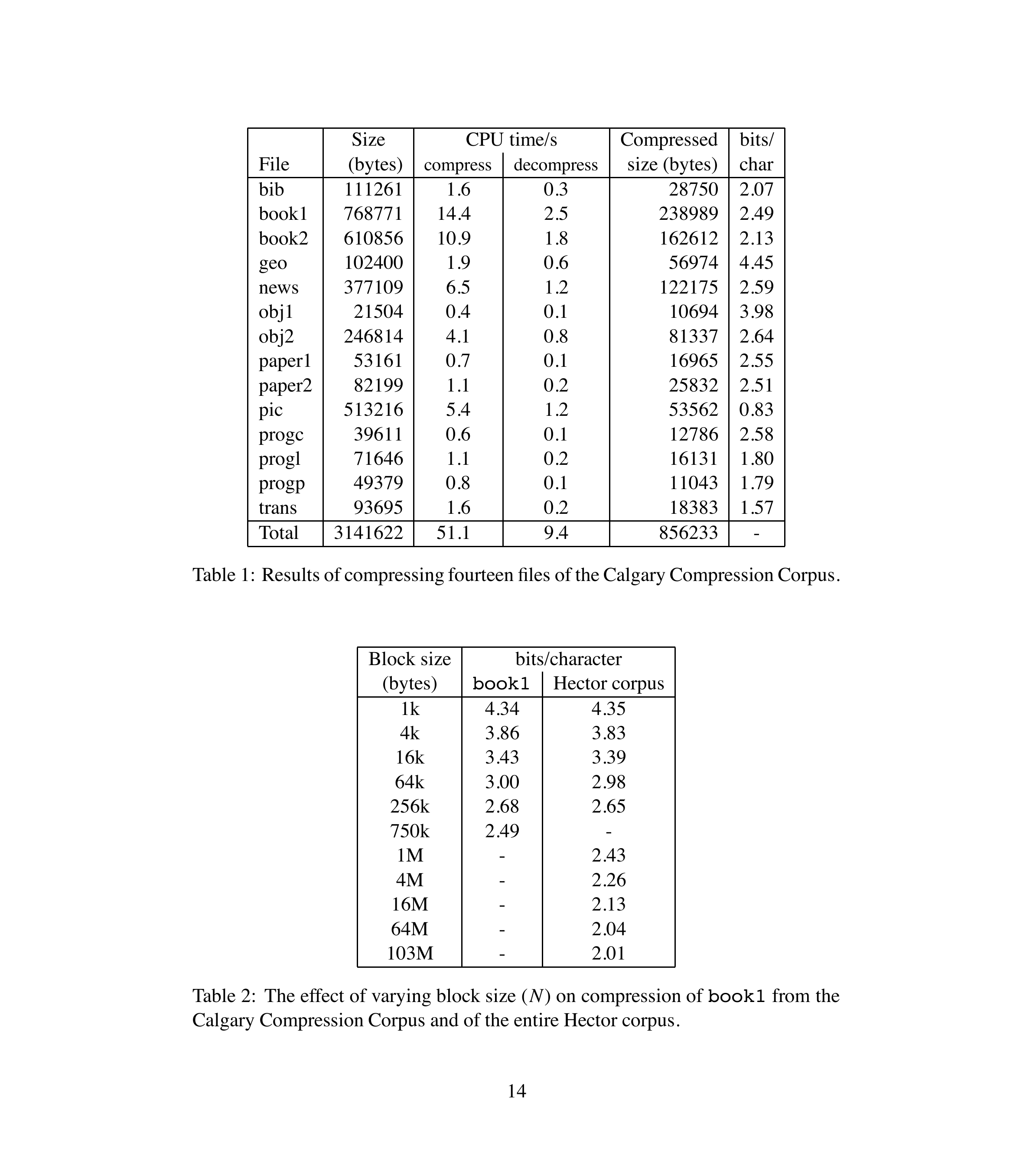
在表 1中,我们给出了使用本文算法压缩 Calgary 压缩语料库 [7] 的 14 个常用文件的结果。将这些数据与 Bell、Witten 和 Cleary [3] 给出的数据对比可以看出,我们的算法在非文本输入和文本输入上都有良好表现。
我们对算法 C 的实现使用了第 4.1 节描述的技术,并配以简单的移至前端编码器。在每种情况下,块大小 N 都是被压缩文件的长度。
我们用一个修改过的 Huffman 编码器压缩移至前端编码器的输出,该编码器使用了第 5 节描述的技术。我们的编码器为每个 16 KB 输入块重新计算 Huffman 树,而不是为整个输入计算一棵树。
在表 1 中,压缩效率以每输入字符的输出比特数表示。CPU 时间的测量是在 DECstation 5000/200 上进行的,该机器配备 MIPS R3000 处理器,主频 25MHz,64KB 缓存。这里给出的是 CPU 时间而非墙上时间,以排除执行 I/O 所花的时间。
表 2 显示了对两个输入在不同块大小下压缩效果的变化。第一个输入是 Calgary 压缩语料库中的 book1 文件。第二个是完整的 Hector 语料库 [8],包含稍多于 100 MB 的现代英语文本。结果表明,即使块大小已经相当大时,压缩效果仍然随着块大小的增加而持续改善。然而,将块大小增加到几千万个字符以上时,效果只有很小的提升。
如果块大小无限增大,我们预计算法不会逼近理论最优压缩,因为我们简单的逐字节移至前端编码器会引入一些损失。更好的编码方案也许能在渐近意义上达到最优压缩,但这可能没有太大的实际意义。
📄 原文
In Table 1 we give the results of compressing the fourteen commonly used files of the Calgary Compression Corpus [7] with our algorithm. Comparison of these figures with those given by Bell, Witten and Cleary [3] indicate that our algorithm does well on non-text inputs as well as text inputs.
Our implementation of Algorithm C uses the techniques described in Section 4.1, and a simple move-to-front coder. In each case, the block size N is the length of the file being compressed.
We compress the output of the move-to-front coder with a modified Huffman coder that uses the technique described in Section 5. Our coder calculates new Huffman trees for each 16 kbyte input block, rather than computing one tree for its whole input.
In Table 1, compression effectiveness is expressed as output bits per input character. The CPU time measurements were made on a DECstation 5000/200, which has a MIPS R3000 processor clocked at 25MHz with a 64 kbyte cache. CPU time is given rather than elapsed time so the time spent performing I/O is excluded.
In Table 2, we show the variation of compression effectiveness with input block size for two inputs. The first input is the file book1 from the Calgary Compression Corpus. The second is the entire Hector corpus [8], which consists of a little over 100 MBytes of modern English text. The table shows that compression improves with increasing block size, even when the block size is quite large. However, increasing the block size above a few tens of millions of characters has only a small effect.
If the block size were increased indefinitely, we expect that the algorithm would not approach the theoretical optimum compression because our simple byte-wise move-to-front coder introduces some loss. A better coding scheme might achieve optimum compression asymptotically, but this is not likely to be of great practical importance.
与其他压缩程序的比较
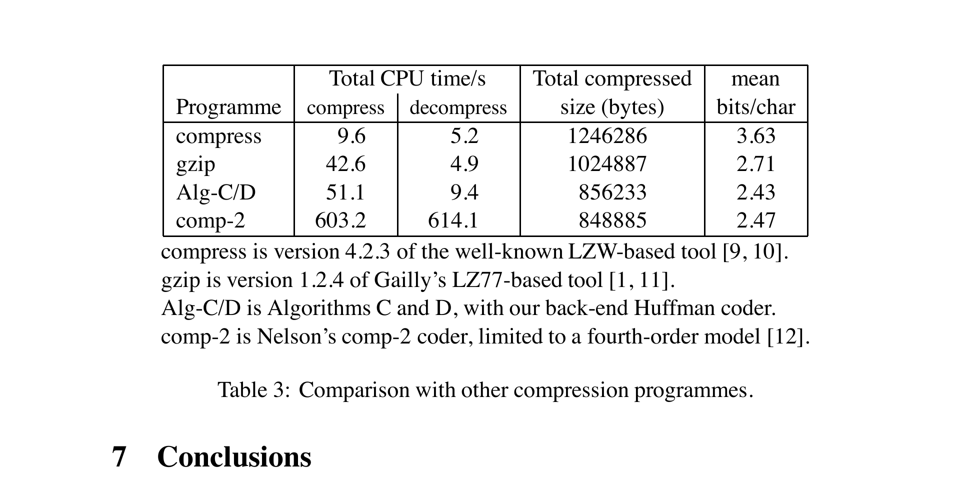
表 3 将本文实现的算法 C 与另外三个压缩程序进行比较,这些程序因其广泛可用性而被选中。对同样的 14 个文件,每个算法分别单独压缩,再将结果相加。每字符比特数是各文件数值的平均值。之所以选择这个指标,是为了便于与 Bell [3] 给出的数据进行比较。我们的算法在压缩率上显著优于 compress(LZW)和 gzip(LZ77),接近最优的统计建模方法,而速度更接近基于 Lempel-Ziv 的算法。
📄 原文
Comparison with other compression programmes
Table 3 compares our implementation of Algorithm C with three other compression programmes, chosen for their wide availability. The same fourteen files were compressed individually with each algorithm, and the results totalled. The bits per character values are the means of the values for the individual files. This metric was chosen to allow easy comparison with figures given by Bell [3].
📖 深入解析
性能数据的核心看点:
- 压缩率:在 Calgary 语料库 14 个文件(总计 3,141,622 字节)上,BWT 算法压缩到 856,233 字节,约 2.43 位/字符。相比之下,compress(LZW)需要 3.63 位/字符,gzip 需要 2.71 位/字符。BWT 的压缩率接近四阶统计建模 comp-2 的 2.47 位/字符。
- 速度:压缩 51.1 秒,解压仅 9.4 秒(gzip 为 42.6 秒压缩)。解压不对称性是 BWT 的一大优势——适合"一次压缩、多次解压"的场景。
- 块大小效应:块越大压缩越好。对 book1 文件,1KB 块时 4.34 位/字符,256KB 块时降至 2.68 位/字符。对 Hector 语料库(约 100MB 英文),64MB 块时达到 2.04 位/字符。这说明 BWT 能利用的上下文范围随块大小增长而扩大。
- 代价:BWT 需要将整个块装入内存才能排序,不适合流式数据。大块的排序也是最耗时的步骤——这是 BWT 先天的时间-空间权衡。
25MHz 的 R3000 处理器上 51.1 秒压缩 3MB——用今天的标准看很慢,但在 1994 年是实用的。
7. 结论
我们描述了一种压缩技术,它通过对文本块施加可逆变换,使输入中的冗余性更易于被简单编码方案利用。我们的算法是通用型的,在文本和非文本输入上均表现良好。该变换通过排序将基于上下文的字符聚集在一起;该技术利用了每个字符仅一侧的上下文信息。
要获得良好的压缩效率,需要数千字符的输入块。算法的有效性随着块大小的增加而持续改善,至少在达到数百万字符之前都是如此。
我们的算法实现了与优秀的统计建模器相当的压缩率,而速度更接近基于 Lempel-Ziv 算法的编码器。与 Lempel-Ziv 算法一样,我们的算法解压快于压缩。
📄 原文
7. Conclusions
We have described a compression technique that works by applying a reversible transformation to a block of text to make redundancy in the input more accessible to simple coding schemes. Our algorithm is general-purpose, in that it does well on both text and non-text inputs. The transformation uses sorting to group characters together based on their contexts; this technique makes use of the context on only one side of each character.
To achieve good compression, input blocks of several thousand characters are needed. The effectiveness of the algorithm continues to improve with increasing block size at least up to blocks of several million characters.
Our algorithm achieves compression comparable with good statistical modellers, yet is closer in speed to coders based on the algorithms of Lempel and Ziv. Like Lempel and Ziv's algorithms, our algorithm decompresses faster than it compresses.
📖 深入解析
1994 年这篇报告发表时主要被视为一个优秀的压缩算法,但其历史意义远超压缩领域:
- 2000 年:Ferragina & Manzini 发现 BWT + C 数组 + O 数组可以构成全文索引 → FM-index,可在 O(p) 时间内完成精确模式匹配
- 2009 年:Li & Durbin 将 FM-index 用于 DNA 短读段比对 → BWA,使人类基因组规模的短读段比对成为实用
- 今天:BWT/FM-index 是几乎所有主流 DNA 比对工具(BWA、Bowtie、SOAP2、STAR、Salmon)的核心数据结构
论文中"只利用了字符一侧的上下文"这一限制,在生物信息学中反而成了优势:参考基因组序列的 BWT 只需构建一次,查询模式串的前缀即可确定匹配的后缀数组区间。这种单向性恰好与 DNA 读段的比对需求吻合。
一篇原本为压缩而写的技术报告,时隔 15 年成为基因组学的基石——这是计算机科学中"基础研究催生意想不到的重大应用"的经典案例。